Towards a Gradient Syntactic Model for Unsupervised Parsing
A PhD dissertation draft
You can find the .pdf version here.
Abstract
Currently, the world stores and exchanges unprecedented amounts of information in the form of text; however, although we also have unprecedented amounts of computing power, our ability to process this information is limited by our ability to computationally decode the grammar of human language. There are, in fact, algorithms that can recognize syntactic patterns in language, and learn to do so for any language, by training on text samples alone, without referencing the correct syntactic analyses. Such algorithms are called unsupervised parsers.
Unsupervised parsers do not perform well enough yet for widespread use. Most work by assuming that the unruly probabilistic patterns of language are generated by much simpler hidden syntactic structures. To infer these hidden structures, the parsers first observe words in the training text, then infer the underlying syntactic structure — usually a phrase-structure tree or a dependency tree — that most likely generated each sentence. These results are then evaluated against syntactic structures annotated by human linguists. This has proven to be a difficult task. Inference techniques have become increasingly sophisticated, but performance has yet to improve significantly.
Rarely explored is the possibility that the problem may lie in the oversimplicity of the syntactic structures themselves. The conventional approach imposes clean categories onto the messy complexity of human language, forcing words with different syntactic behaviour into uniform parts of speech, labeling phrases with different properties as constituents, and recognizing different kinds of syntactic relations as dependencies. The resulting categories and structures may be simple in form, but their diverse membership make them difficult to either identify or interpret. Indeed, disagreement over such analyses is common even among linguists, whose analyses form the “gold-standard” that parsers are evaluated against.
What we need is a model that can describe greater variation with simple, precisely-defined concepts. To this end, I propose the Gradient Syntactic Model. Instead of parts of speech, this model measures the degree of similarity between words based on the number of shared contexts. Each word has a unique neighbourhood of words whose similarity to it lies within a certain threshold. The model also quantifies the coherence of phrases, by comparing their relative frequencies to what they would be if their component words occurred independently. Besides also having neighbourhoods, phrases have two similarity metrics. Lastly, the model measures conditional probabilities between all combinations of words, phrases, and their neighbourhoods. These are used to calculate the sentence’s grammaticality score.
The Gradient Syntactic Model provides a gradient analysis much richer than discrete structures, based on well-defined concepts. It is by no means complete, and much work remains. Nevertheless, it points out a new way forward in unsupervised parsing, towards the use of gradient models that are better suited to natural language processing.
Preface
While this thesis draft was never defended, and did not help me graduate, I would still like to share it. For one thing, I spent more than three years on it. But more importantly, it develops an idea whose value I still believe in strongly: that using quantitative gradient measures, in place of conventional categories and binary relations, can increase the predictive power of linguistic models, and allow them to power the use of natural (human) language by machines.
Conventional discrete models were designed to help linguists analyze and compare language structure. They do this by simplifying the complexity of language, providing a high-level but low-resolution view. Today, computational algorithms that analyze grammatical structure, known as parsers, still mostly rely on these discrete models. But in terms of power, these models cannot compare to the language models in our brains, which allow us to actually produce and understand language on a daily basis.
Since I began this work in 2014, many exciting developments have taken place in the field of language modeling. In February 2019, the research institute OpenAI released GPT-2, a deep-learning language model that can reportedly create astoundingly coherent pieces of writing, just by starting from a short phrase or sentence and then continuously predicting the next word. While commercial applications are still elusive, the potential of this technology is great, to the point of being somewhat unsettling.
Meanwhile, this quantitative, non-discrete approach to language structure is not only useful technologically, but can also greatly improve our understanding of linguistics. A high-resolution model can reveal patterns and relationships hidden by low-resolution discrete models. It also forces us to be more precise about concepts such as grammatical relations, parts of speech, and word boundaries.
This thesis draft is just an exploratory first step in this direction. There is a lot of work to be done. I am putting my work here on Medium, in the hopes that it might find its way to others who can use it to work towards a better understanding of syntax. That, to me, would be a bigger accomplishment than getting a degree.
Table of Contents
Abstract
Preface
Abbreviations: Penn Treebank Tagset
1 Introduction
1.1 The usage-based approach
1.2 Goal and scope of thesis
1.3 Outline of dissertation
2 Current models in unsupervised parsing
2.1 Parts of speech
2.1.1 In linguistic description
2.1.2 In unsupervised POS-induction algorithms
2.1.3 In unsupervised parsing
2.2 Syntactic relationships
2.2.1 Constituents in linguistic descriptions
2.2.2 Dependencies in linguistic descriptions
2.2.3 Constituents and dependencies in unsupervised parsing
2.3 Rethinking discrete syntactic models
3 Gradient Syntactic Model
3.1 Lexical-syntactic behaviour
3.1.1 Contextual similarity
3.1.2 Evaluation
3.1.3 Discussion
3.2 Phrases
3.2.1 Phrasal coherence
3.2.2 Phrasal comparison
3.3 Conditional probabilities
3.3.1 Conditional probabilities
3.3.2 Grammaticality
3.3.3 Evaluation
4 Conclusions
4.1 Contributions
4.2 The road ahead
References
List of Tables
Table 2.1: Span, label, and context of every constituent in the sentence Factory payrolls fell in September (taken from Klein and Manning 2002:129)
Table 2.2: Performance of various baselines and systems, on various parts of the WSJ corpus (Klein and Manning 2004, Bod 2009, Spitkovsky et al. 2013)
Table 3.1: Context sets for the words replace, affect, and school, from Penn Treebank-3
Table 3.2: Shared contexts among replace, affect, and school
Table 3.3: Jaccard Distances among replace, affect, and school
Table 3.4: Jaccard Distances and POS tags for the closest ten neighbours of each of the ten words chosen for evaluation
Table 3.5: Frequency information and context sizes of the ten words chosen for evaluation, in order from most to least frequent
Table 3.6: Repeated sequences of lengths 2–4 with the highest SPMIs in Penn Treebank-3
Table 3.7: Phrases in the sentence, “The luxury auto maker last year sold 1,214 cars in the U.S.”
Table 3.8: 10 phrasal neighbours with the lowest Jaccard Distances to the noun phrase “the summer”
Table 3.9: 10 phrasal neighbours with the lowest Jaccard Distances to the infinitival verb phrase “to find”
Table 3.10: 10 phrasal neighbours with the lowest Jaccard Distances to the adjective phrase “more difficult”
Table 3.11: Frequency, context set size, and maximum number of possible matches for the five phrases chosen for evaluation
Table 3.12: 10 phrasal neighbours with the lowest Jaccard Distances to the adverbial phrase/adjective phrase “very much”
Table 3.13: 10 phrasal neighbours with the lowest Jaccard Distances to the prepositional phrase “in the u.s.”
Table 3.14: 10 phrasal neighbours with the lowest Jaccard Distances to the prepositional phrase “in the u.s.,” without redundant contexts
Table 3.15: 10 phrasal neighbours with the lowest sequential distances to the noun phrase “the role”
Table 3.16: 10 phrasal neighbours with the lowest sequential distances to the verb phrase “has n’t been set”
Table 3.17: 10 phrasal neighbours with the lowest sequential distances to the adjective phrase “partly responsible”
Table 3.18: 10 phrasal neighbours with the lowest sequential distances to the adverbial phrase “more closely”
Table 3.19: 10 phrasal neighbours with the lowest sequential distances to the prepositional phrase “in the u.s.”
Table 3.20: 20 sentences used in the evaluation of conditional probabilities and grammaticality scores
Table 3.21: Phrases in the sentence, “They thought it would never happen.”
Table 3.22: Conditional probability ratios between all pairs of elements or their neighbourhoods in Sentence 1
Table 3.23: Grammaticality scores of the 20 sentences in the evaluation
List of Figures
Figure 2.1: Illustration of an example of an EM algorithm (taken from Do and Batzoglou 2008)
Figure 2.2: A constituency tree for the sentence Factory payrolls fell in September (taken from Klein and Manning 2002:129)
Figure 2.3: The collection of trees and subtrees generated in U-DOP for the sentences watch the dog and the dog barks (taken from Bod 2009:762)
Figure 2.4: A dependency tree for the sentence factory payrolls fell in September (Klein and Manning 2002:129)
Figure 2.5: Steps in the derivation of the dependency tree in Figure 2.4, in DMV
Figure 2.6: Three kinds of parse structures (taken from Klein and Manning 2004:129)
Figure 3.1: Precisions at K for the ten words chosen for evaluation
Figure 3.2: How Jaccard Distances are used to calculate sequential distances Figure 3.3: Grammaticality scores of the 20 sentences in the evaluation
Figure 3.4: Visual representation of gradient analysis, Sentence 1
Figure 3.5: Combined representation of phrase structure and dependency analyses, Sentence 1
Figure 3.6: Gradient and discrete analyses of the 20 evaluated sentences
Abbreviations: Penn Treebank Tagset
The following is a list of the part-of-speech tags used in the Penn Treebank:
ᴄᴄ — Coordinating conjunction
ᴄᴅ — Cardinal number
ᴅᴛ — Determiner
ᴇx — Existential there
ꜰw — Foreign word
ɪɴ — Preposition or subordinating conjunction
ᴊᴊ — Adjective
ᴊᴊr — Adjective, comparative
ᴊᴊꜱ — Adjective, superlative
ʟꜱ— List item marker
ᴍᴅ — Modal
ɴɴ — Noun, singular or mass
ɴɴꜱ — Noun, plural
ɴɴᴘ — Proper noun, singular
ɴɴᴘꜱ — Proper noun, plural
ᴘᴅᴛ — Predeterminer
ᴘoꜱ — Possessive ending
ᴘʀᴘ — Personal pronoun
ᴘʀᴘ$ — Possessive pronoun
ʀʙ— Adverb
ʀʙʀ— Adverb, comparative
ʀʙꜱ— Adverb, superlative
ʀᴘ— Particle
ꜱʏᴍ — Symbol
ᴛo — to
ᴜʜ — Interjection
ᴠʙ — Verb, base form
ᴠʙᴅ — Verb, past tense
ᴠʙɢ — Verb, gerund or present participle
ᴠʙɴ — Verb, past participle
ᴠʙᴘ — Verb, non-3rd person singular present
ᴠʙz — Verb, 3rd person singular present
wᴅᴛ — Wh-determiner
wᴘ — Wh-pronoun
wᴘ$ — Possessive wh-pronoun
wʀʙ — Wh-adverb
«Il ne faut pas avoir peur d’aller trop loin, car la vérité est au-delà.»
“We must never be afraid to go too far, for truth lies just beyond.”
— Marcel Proust
1 Introduction
In the last few decades, as computer and internet usage has become increasingly widespread, a vast quantity of information in the form of digitized text has become readily available. This has led to the increasing popularity of corpus linguistics, the study of language through the analysis of language corpora. No longer do linguists have to rely solely on intuition to judge the prevalence of grammatical patterns.
There remains, however, a need for tools that can enable more sophisticated forms of corpus analysis. In particular, there is currently still no reliable way of automatically identifying syntactic patterns in unannotated corpora. For example, to determine how many uses of a certain verb are transitive and how many are intransitive, linguists must still rely on manual annotation. For many languages without access to linguistic resources, this is not a readily-available option.
One tool that can satisfy this need is parsers, algorithms that analyze the syntactic structure of sentences. Among parsers, those that can train on unannotated corpora are known as unsupervised parsers. Unsupervised parsers can be deployed in any language for which raw text is available in large quantities.
They carry enormous potential both for our understanding of language and for our ability to process it. For linguistics, they can facilitate the development of syntactic theories by providing a way to test hypotheses. This feedback, which is currently lacking, is essential for improving our understanding of linguistics.
On the technological side, the applications of unsupervised parsers are numerous. With the increase in the quantity of digitized text comes the need for tools to help process it. Current natural language processing (NLP) tools, such as search engines and machine translators, do make use of statistical properties of words and phrases; however, so far they have not been able to take advantage of syntactic structure. A syntactic model can significantly boost the effectiveness of these existing tools. Machine translation results can become more coherent; search engines can recognize queries as coherent phrases or sentences, instead of merely a structureless string of words; information extraction algorithms can better identify relationships between entities in sentences; and so on.
Despite significant improvements since the beginning of their development in the early 1990s, unsupervised parsers are not yet widely used. One major obstacle to their progress is their reliance on discrete syntactic models. In these discrete models, words are classified into part-of-speech categories, then either grouped into nested phrases to form phrase-structure trees, or put into dependency relations to form dependency trees. All three concepts — parts of speech, phrases, and dependencies — are discrete: a word either belongs to a part-of-speech, or it does not; either a sequence of words forms a phrase, or it does not; either a word is in a dependency relationship with another word, or it is not.
This discrete approach may be adequate in descriptive linguistics, where linguistic analyses are designed to be understood by human readers. However, it is ill-suited for parsers, whose output is meant to be used by other NLP applications. First, in order to fit language into neat discrete categories and relationships, discrete models discard information that is vital to an accurate analysis. Second, the analyses constructed by discrete models are based on higher-level and vaguely-defined concepts. In short, it takes detailed measurements from text, then simplifies them to create an ill-defined analyses.
Both NLP and linguistics can benefit greatly from reliable unsupervised parsers. To achieve this, we need a more precise model of syntax that can take full advantage of the large amount of linguistic data currently available. It is to this end that I propose the Gradient Syntactic Model.
1.1 The usage-based approach
A major inspiration for the Gradient Syntactic Model is the usage-based approach in linguistics, as exemplified by Bybee (2010). The usage-based approach views language as a dynamic process, rather than a static structure. Bybee (2010) illustrates in detail how this dynamic view of language can account for both diachronic changes in linguistic structures and their synchronic variation.
This model of language as a dynamic process leads naturally to the concept of gradience in linguistic structure. As Bybee (2010:1) writes, “Language is … a phenomenon that exhibits apparent structure and regularity of patterning while at the same time showing considerable variation at all levels.” While giving the illusion of discreteness, language patterns are in reality gradient and context-dependent. For example, differences in lexical-syntactic behaviour are not categorical, as parts of speech suggest; Bybee shows how auxiliaries in English diverged from finite verbs gradually, through the gradual increase in the usage frequencies of modals and the verbs be, have, and do (120–135). Meanwhile, phrases and morphologically-complex words vary in their degree of unity, depending on how their frequencies as a unit compare to the frequencies of their component morphemes (46–50). Thus, it is through gradient differences that both synchronic variations and diachronic changes occur.
The usage-based approach thus inspires the use of gradient syntactic models in unsupervised parsing. Gradient syntactic models offer at least two major improvements to conventional syntactic models. First, by recognizing gradient rather than categorical differences between words and phrases, they provide greater descriptive power. Discrete structures can be described precisely with a gradient model, but gradient structures often cannot be described by discrete models without loss of information. Second, by using gradience to account for complexity, gradient models can use quantitative concepts that are easier to define. For example, in a discrete phrasal analysis, a phrase is either a constituent or not. However, this decision is based on many different criteria which are not necessary and sufficient, and which serve more as guidelines. Thus, discrete phrasal analyses leave room for uncertainty. In contrast, in a gradient model, phrases (called chunks in Bybee 2010) are given much more room to vary; specifically, they can vary in their frequency of occurrence relative to those of their component words. The higher the relative frequency of a chunk is, the stronger it can be judged as a unit. This gradient variation is much greater than the binary choice between constituency and distituency, but in return it is much precisely-defined.
With its use of precisely-defined quantitative measurements, the usage-based approach is a natural fit for a computational syntactic model. This dissertation, then, is an exploration of this possibility.
1.2 Goal and scope
The Gradient Syntactic Model is a first attempt at a new kind of syntactic model, one that is designed for natural language processing rather than human readers. It aims to use only precisely-defined concepts, in order to predict syntactic patterns as accurately as possible. Together, these two design goals lead to a model that uses a small number of simple, rigorously-defined gradient relationships to capture a large number of syntactic patterns.
The version of the Gradient Syntactic Model described and implemented in this dissertation is meant to be a feasibility study and prototype, rather than a definitive model. There are several limitations to the current model. The first is the size of the training corpus. In order to speed up the development process, the training corpus (Penn Treebank-3) was deliberately chosen to be small (933,886 tokens). This, however, necessarily affects the model’s performance. Of course, much larger corpora are available, and once the implementation has been better optimized, it can hopefully be trained on significantly more data.
In addition, the lack of standard gradient analyses makes evaluation challenging. The Gradient Syntactic Model is designed to measure different information from conventional discrete models, and so their analyses are difficult compare. An ideal evaluation for the Gradient Syntactic Model would measure the performance boost it lends to other NLP applications; however, this lies outside our current scope. Nevertheless, in some places, we can gauge the quality of gradient analyses by examining how well they align with discrete analyses and expected results. Towards the end, we will evaluate the gradient model comprehensively by rating the grammaticality of sentences with a grammaticality score, then judging how well this grammaticality score differentiates between grammatical and ungrammatical sentences.
Thirdly, as implied in its name, the Gradient Syntactic Model only models syntactic relationships, those between words in a sentence. It therefore excludes all other areas of language — phonetics, phonology, morphology, semantics, and pragmatics — though some non-syntactic information may be captured indirectly. Since syntax interacts with all these other aspects of linguistics to some degree, the syntactic analysis that this model can provide will not be complete.
Finally, although this dissertation describes the implementation of a linear training process, the training of the Gradient Syntactic Model was originally conceived as an iterative process. The training process described herein constitutes only the first iteration of training. In subsequent iterations, the model can be improved by incorporating measurements and analyses made in the first one. Unfortunately, due to time constraints, this iterative training process will have to be implemented in the future.
Many other areas in the Gradient Syntactic Model can be further development; the most important ones will be discussed in the Conclusion. The main purpose of this dissertation, however, is to lay the foundation for the Gradient Syntactic Model. The task of revealing the model’s full potential will be left to future efforts.
1.3 Outline of dissertation
Chapter Two describes conventional discrete syntactic models, and how they have been used in unsupervised parsing. In the process, it will also examine the model’s appropriateness for unsupervised parsing. Next, Chapter Three describes the Gradient Syntactic Model by dividing it into three modules: Lexical-Syntactic Similarity, Phrases, and Conditional Probabilities. For each module, it describes the metrics and concepts that are used, presents results from its implementation, and evaluates these results. Finally, Chapter Four offers a general assessment of the entire model, and points out directions for further expansion of the model in the future.
2 Current models in unsupervised parsing
Most unsupervised parsers are based on discrete syntactic models that rely on three concepts from linguistics: parts of speech, constituents, and dependencies. Parts of speech categorize words based on their morphological, syntactic, and semantic properties. Constituents and dependencies indicate syntactic relationships between words: constituents are sequences of words (usually contiguous) that behave as a unit, while dependencies are syntactic relationships between pairs of words, one being the head, and the other its dependent.
As widely used as discrete models are in unsupervised parsing, they were originally developed for quite a different purpose. In linguistics, the purpose of these models has been to provide a theoretical framework for the description of syntax. They were developed for no purpose other than linguistic description, though sometimes they were incorporated as a part of more comprehensive theories of language, such as Generative Grammar. By the time these models were adapted to unsupervised parsing, they had already been used by linguists for some time, from almost a century in the case of constituents, to several millennia in the case of parts of speech.
For linguistic description, discrete models have their advantages: they are intuitive and easy to grasp, and they can be applied to a wide variety of syntactic patterns in languages with very different typology. However, as models in unsupervised parsers, they have two serious drawbacks: being discrete, they oversimplify the heterogeneity of the patterns they try to describe; and, being high-level, they are complex and difficult to define precisely. Together, these problems not only make discrete structures difficult for algorithms to infer, but also severely limit their usefulness. Unsupervised parsers are thus given the task of simplifying rich linguistic data in a complex yet ill-defined way.
In this chapter, we will discuss the three discrete linguistic structures currently used in unsupervised parsers: parts of speech, constituents, and dependencies. We will also see how these structures are used by unsupervised POS-induction algorithms and unsupervised parsers, using previous work to illustrate. We will compare the performances of some of this previous work, stretching back to the early days of NLP. Finally, informed by the history of the problem and its proposed solutions, we will revisit the question of the appropriateness of discrete models for the task of unsupervised grammar induction, and discuss the way forward.
2.1 Parts of speech
Parts of speech are categories of words that share morphological, syntactic, and semantic properties. Their use in linguistics stretches back millennia, and they are currently still widely used both in linguistics and in NLP, including in unsupervised parsing. However, the convenience of using discrete categories to characterize lexical properties comes at the cost of obscuring both differences between words within categories and differences between categories.
In this section, we will investigate the nature of parts of speech and their suitability for unsupervised parsing. Additionally, we will examine how unsupervised part-of-speech induction algorithms infer parts of speech. These algorithms provide a starting point for the learning of lexical properties in the Gradient Syntactic Model.
2.1.1 In linguistic description
Words in a language exhibit a variety of morphological, syntactic, and semantic properties, which are collectively referred to as lexical properties, or lexical behaviour. Though lexical properties do not generally fall neatly into categories, some of them can be used to group words into a small number of categories, which we now know as parts of speech. Through categorization (or more generally, generalization), parts of speech provide a convenient way of describing the properties of a word. This is especially useful for words that occur too rarely for enough information to be gathered about them.
As far back as the 5th century BC, the ancient Sanskrit grammarian Yāska classified Sanskrit words into four main parts of speech: nouns (nāma), verbs (ākhyāta), verbal prefixes (upasarga), and invariant particles (nipāta) (Matilal 1990). Later, in a treatise called The Art of Grammar dating from the 2nd century BC, the Greeks came up with eight parts of speech: nouns, verbs, participles, articles, pronouns, prepositions, adverbs, and conjunctions. With only a few minor modifications, these categories have remained as parts of speech used for English today. In Generative Grammar (e.g. Radford 1988), parts of speech — or “word-level categories” — came to be modeled in Universal Grammar as underlying categories, to which all words in all languages fundamentally belong.
But while it is always possible to categorize words by their lexical properties, these resulting categories are often quite difficult to define. Beck (2002) examines the advantages and disadvantages of categorizing words using morphological, syntactic, or semantic properties alone. To the untrained observer, out of all the different kinds of lexical properties, semantic properties are the most salient. For example, a noun is commonly described as a “person, place, or thing,” while a verb is typically thought of as an “action word.” But while such descriptions do fit the most typical examples of nouns and verbs (e.g. tree for nouns, and run for verbs), many words do not fit these descriptions. Many nouns do not refer to people, places, or things, but instead refer to qualities, such as warmth, or ideas, such as democracy. Similarly, many verbs describe events that are not actions, but states; examples include be, have, and endure. More importantly, a categorization scheme based on language-independent semantic properties alone would neglect language-specific morphosyntactic properties, something that parts of speech were designed to do in the first place.
It is also problematic to define parts of speech solely by morphosyntactic properties. Here we run into the opposite problem: morphosyntactic properties are language-specific, yet parts of speech such as nouns and verbs are identified in many different languages. The fact that words in different languages can be identified as nouns suggests that they share some semantic characteristics. Relying solely on morphosyntactic properties to define parts of speech neglects their striking semantic similarities.
The fact that similar parts of speech have been identified in a wide variety of languages reflects a strong tendency for language-specific lexical-morphosyntactic properties to align with language-general lexical-semantic properties. Only semantic properties are shared across languages, while morphosyntactic properties pertain to specific languages. But it is the association of morphosyntactic properties with similar semantic properties that give rise to similar parts of speech across languages. Theoretically, this generality is far from inevitable — we could easily imagine an alternate scenario where lexical-morphosyntactic properties had little correlation with lexical-semantic ones. In that case, all parts of speech would necessarily be language-specific.
Thus, Beck (2002) finds that even though parts of speech can be compared cross-linguistically, neither morphology, syntax, nor semantics is sufficient by itself to adequately define each part of speech cross-linguistically. To remedy this, he proposes definitions for nouns, verbs, and adjectives that make use of both semantic and syntactic criteria (morphological criteria were left out because morphology is not significant in all languages). A noun, for example, is defined as an element expressing a semantic name — “a conceptually-autonomous meaning referring to an individual, discrete, or abstract entity” — which can be a syntactic dependent without further measures (76–78). (Syntactic heads and dependents will be discussed later in the chapter, in the description of dependencies.)
Such definitions are sufficiently precise for linguistic analyses written for human readers. However, for unsupervised part-of-speech (POS) induction algorithms, these definitions are conceptually too high-level. Algorithms — at least initially — cannot determine if a word is “conceptually-autonomous,” having no access to this level of semantics; nor, as unsupervised algorithms, do they have information about whether a word is a syntactic head or dependent, since this requires access to dependency trees. Similarly high-level information would be required to determine if an element can be a head or a dependent without further measures.
For a computational model of lexical properties, a different approach is therefore necessary. Since high-level computational semantic models are not yet available, in the meantime, a computational lexical model should leave out semantic properties, and focus on morphosyntactic properties. Furthermore, since computational models are capable of storing vast numbers of precisely quantified relationships, they would not need to rely on discrete categories to simplify the great variety of lexical properties in a language, as humans do.
A glimpse of a possible alternative can be seen in Bybee (2010). Instead of treating parts of speech as discrete categories and attempting to establish criteria for them, Bybee (2010) adopts a more emergent view of parts of speech. To her, words are fundamentally heterogeneous, but share similarities that suggest family resemblance structures (Wittgenstein 1953). Some words can be considered more typical of a pattern, while others are more marginal, depending on the relative frequency with which they display the properties shared by other words in the same part of speech. None of these properties, however, are necessary or sufficient for membership. Parts of speech are not seen as fundamental static categories, but rather emergent categories that are constantly in flux.
As we will see, this view of parts of speech is more in line with the strategies used in unsupervised POS induction algorithms, which infer parts of speech from unannotated corpora.
2.1.2 In unsupervised POS-induction algorithms
While linguistic definitions of parts of speech are conceptually too high-level to be useful in algorithms, computational linguists have found other ways to infer parts of speech, using information that algorithms have ready access to. Most unsupervised POS-induction algorithms employ one of three general strategies. The first strategy can be described as an optimal classification search. An algorithm starts off with some initial categorization, the simplest of which is to place each word in its own word class. Then, a word is moved to another category, if doing so leads to an improvement; an improvement is usually defined as an increase in the probability of the training text. The probability of each word in the text, assuming a bigram model, can be calculated with the formula

where wᵢ is the word in position i in a sentence, and cᵢ is the word class of wᵢ (Brown et al. 1992). Two notable algorithms that employ this general strategy are Brown et al. (1992) and Clark (2003), the former being the earliest POS-induction algorithm of note in the literature. Both algorithms seek to find a categorization that maximizes the probability of the training corpus. Both algorithms assume some fixed number of word classes.
The second strategy, which I will call context vector clustering, is exemplified by Finch and Chater (1992) and Schütze (1995). In Schütze (1995), the 250 most frequent words in the training data are used as context words. Then, the algorithm records the number of times each of those context words occurs immediately on the left or right of each of the remaining words in corpus, so that each of these words has a left and right context vector. These left and right context vectors are then concatenated into 500-dimensional vectors, which is then reduced to 50-dimensional vectors using SVD (Singular Value Decomposition, a method of dimension reduction). These 50-dimensional vectors are finally clustered into 200 word classes. Similarly, to classify high- and medium-frequency words, Biemann (2006) uses the 200 most frequent words in the training corpus as context words, and characterizes each word by the number of times these context words occur immediately on the left and right of it. However, his algorithm clusters words somewhat differently, by putting each word into the class whose members have the greatest total similarity score to it. This way, the number of clusters does not need to be predetermined.
The third strategy uses Hidden Markov Models, or HMMs (see Blunsom 2004 for an introduction). One of the earliest unsupervised parser to use an HMM is Merialdo (1994), who implements a trigram HMM. The trigram HMM makes two approximations: that the probability of each part-of-speech tag depends only on the tags of the previous two words, and that the probability of each word depends only on its POS tag. The algorithm then chooses the POS tags that maximize the likelihood of the training corpus. More recent efforts tend to combine HMMs with more sophisticated machine-learning techniques, and can be described as augmented HMMs; these include Goldwater and Griffiths (2007), Johnson (2007), Graca et al. (2009), and Berg-Kirkpatrick et al. (2010).
Which strategy holds the most promise, and how well does it do? Christodoulopoulos et al. (2010) provide a careful evaluation of representative studies over the previous two decades, performing benchmark tests on seven unsupervised POS-induction algorithms: Brown et al. (1992), Clark (2003), Biemann (2006), Goldwater and Griffiths (2007), Johnson (2007), Graca et al. (2009), and Berg-Kirkpatrick et al. (2010). While each paper provides an evaluation of its own system, Christodoulopoulos et al. (2010) subjects all systems to the same tests. Moreover, in addition to testing the systems on the WSJ corpus, which most of the systems were developed on, the evaluation also tests them on translations of a multilingual corpus, Multext-East, in eight different European languages. After weighing various methods of measuring how well the induced clusters match gold-standard tags, the authors found that an entropy-based metric, V-measure, to be the most reliable (Rosenberg and Hirschberg 2007).
According to the benchmark tests, the algorithm that performs the best on corpora from eight different European languages was Clark (2003), with Brown et al. (1992) and Berg-Kirkpatrick et al. (2010) following close behind. The study also introduces a new method of evaluation. From each cluster induced by each system, words were selected heuristically as prototypes. These prototypes were then fed into another POS-induction system, Haghighi and Klein (2006), which uses these prototypes to induce new clusters. This was partly motivated by the possibility that this method of induction may yield better clusters than each of the algorithms by itself. Here, Brown et al. (1992) emerged as the winner.
Two observations can be made about these benchmark results. First, as the authors note, the older algorithms outperform many of the more recent ones. Brown et al. (1992) and Clark (2003), both employing the first strategy, optimal classification search, are the two oldest systems in the evaluation, yet are among the best performers overall, rivaled only by the newest system that was reviewed, Berg-Kirkpatrick et al. (2010). Second, even the winning systems are fairly limited in their performance. Christodoulopoulos et al. (2010) includes an evaluation of all seven systems on WSJ, which is the corpus that most of the systems were developed on, and which should therefore elicit the best results. Still, none surpasses 70% in V-measure — significantly better than the baseline of grouping each word in its own cluster (35.42%), but still a long way from the 95.98% reached by the Stanford Tagger, a supervised system.
The more recent unsupervised POS taggers, the augmented HMMs, tend to concentrate on refining statistical techniques. The increasing complexity of these techniques is reflected by the runtimes of the systems reported in Christodoulopoulos et al. (2010). While the earlier, non-HMM systems finish within an hour, the augmented HMM systems take anywhere from about 4 hours in the case of Goldwater and Griffiths (2007) to about 40 hours in the case of Berg-Kirkpatrick et al. (2010). Furthermore, the benchmark results suggest that this increase in complexity is not matched by a corresponding increase in performance.
The diminishing returns in the progress of unsupervised POS-tagging calls for some reflection. Parts of speech have been shaped partly by factors that the algorithms have no access to. These considerations include the semantic properties of words, the cognitive biases of linguists who choose which criteria are important, and historical accidents that have influenced how words have been categorized. Meanwhile, POS-induction algorithms only have access to a text corpus. Therefore, there may be a theoretical limit to how closely the results from these algorithms can align with traditional part-of-speech classifications.
It is also important to remember what parsers use parts of speech for. Parsers use them to help learn the syntactic behaviour of low-frequency items, and to focus its attention on the syntactic relationships between words, rather than on the semantic ones. The solution that best serves these purposes may not be the parts of speech that linguists have bequeathed to NLP; indeed, it may not involve categories at all. While categorization has the advantage of simplifying the diversity of lexical behaviour, parsers, unlike human linguists, benefit more from precision than from simplicity. Since every word is to some extent unique, imposing homogeneous categories onto heterogeneous words necessarily obscures their unique properties, thereby compromising precision.
Evidence of the benefits of gradient models comes from Schütze and Walsh (2008), who create a gradient model of lexical-syntactic behaviour using left and right context vectors of each word (termed half-words), similar to Schütze (1995). They first represent sentences in their training data as sequences of these half-words. Then, they use their representations of the sentences to evaluate the grammaticality of unseen test sentences, by determining whether all subsequences of a certain length in the sentence are adequately similar (defined by some threshold) to any sequences stored in training.
In their evaluation, they apply their graded model to 100 grammatical sentences (drawn from the CHILDES corpus, a corpus of conversations with children) and 100 ungrammatical sentences (randomly generated using vocabulary from CHILDES). For comparison, they also build a categorical model based on Redington et al. (1998), in which words are represented by their place in a hierarchical cluster, built based on contextual information similar to Schütze’s half-words. Schütze and Walsh (2008) find that their graded model significantly outperforms the categorical one. These results support the possibility that graded representations of lexical-syntactic behaviour may be more informative than categorical ones, and may in particular lead to better performances in parsing.
2.1.3 In unsupervised parsing
Despite having different goals from descriptive linguistics, unsupervised parsing also relies heavily on parts of speech. Parts of speech provide important information about the behaviour of low-frequency words in training. To learn how words behave syntactically, parsers need to observe repeated instances of them — the more instances the better, since every instance reveals additional information about the word’s behaviour. Parts of speech generalize the properties of high-frequency words to low-frequency words with similar properties, especially lexical-syntactic properties.
Moreover, the lexical-syntactic information provided by parts of speech allows parsers to infer syntactic relationships between words. The frequent co-occurrence of two words in the same sentence is associated not with the existence of a syntactic relationship between the words, but rather with semantic similarity.¹ However, by comparing co-occurrence frequencies of the part-of-speech tags of words rather than of the actual words themselves, unsupervised parsers can more easily infer syntactic relationships and avoid semantic ones. In fact, unsupervised parsers often only use the part-of-speech tags of words in their training corpora, to the exclusion of the actual words themselves. As Spitkovsky et al. (2011) notes, “every new state-of-the-art dependency grammar inducer since Klein and Manning (2004) relied on gold part-of-speech tags.”
One disadvantage in relying on part-of-speech tags is that they generally still require some degree of human effort to produce. Part-of-speech tags in corpora are usually annotated by humans. Alternatively, tags may be generated by supervised tagging algorithms and cleaned up with human labour afterwards. However, these algorithms themselves, being supervised, ultimately still need to train on corpora that are annotated by humans. This reliance on human labour prevents unsupervised parsers from being completely free of human assistance.
Klein and Manning (2005) address this problem by performing their own unsupervised part-of-speech induction, before training their unsupervised parser (CCM, which will be introduced later in the chapter). Using a context-vector clustering strategy similar to Finch and Chater (1992), they cluster the vocabulary in the training corpus into 200 word classes, then use labels for these classes to represent words in training. The result is a noticeably lower F1 score (63.2%) than that achieved with human-annotated POS tags (71.1%), though still above the right-branching baseline F1 score of 60.0%.²
Later, Spitkovsky et al. (2011a) show that inducing parts of speech with an unsupervised system need not lead to worse performance. As a starting point, the authors take their own improved version (Spitkovsky et al. 2011b) of a dependency parser, the Dependency Model with Valence (DMV) (Klein and Manning 2004, which will be described in more detail shortly). They then replace gold-standard POS tags in the training data with labels of word clusters induced by an unsupervised POS-induction algorithm (Clark 2000). The effect of this replacement is only a very slight dip in accuracy. As an additional experiment, they allow words to belong to more than one part of speech, with its part of speech partially-conditioned by its context. Each word has a 10% probability of having its word cluster label replaced by a tag randomly selected from the left-context tags of the following word. With another 10% probability, it receives a tag sampled from the right-context tags of the previous word. Even with this crude approximation of context-sensitivity, accuracy increases, even slightly surpassing the system’s original performance with gold-standard tags (59.1% vs. 58.4%).
¹ This is in fact the principle behind Latent Semantic Analysis: the degree of semantic similarity between two words is indicated by what words they occur with in the same document (which is often taken to be the sentence), and at what frequencies (Deerwester et al. 1990).
² F1 is the harmonic mean of precision and recall, or

2.2 Syntactic relationships
Linguists use various formalisms to represent syntactic analyses, the two most common being constituents and dependencies. Like parts of speech, constituents and dependencies are discrete concepts. More specifically, they are binary relations: two words are either in the same constituent or not, and either in a dependent relationship with each other or not. The simplicity of these two formalisms has made them popular as syntactic models for unsupervised parsers.
However, as with parts of speech, it is difficult to define exactly what constituents and dependencies are, and consequently they are not straightforward to identify. The criteria used to identify them are neither necessary nor sufficient, and sometimes lead to disagreements about the correct analysis. This implies that the phenomena represented by constituents and dependencies are not in fact discrete, but gradient.
2.2.1 Constituents in linguistic descriptions
Intuitively, a constituent is a word sequence, usually (though not always) contiguous, that behaves as a unit. Radford (1988:90), working in the framework of Transformational Grammar (part of the larger theory of Generative Grammar), proposes eight diagnostics for constituency, which tests whether or not a word sequence behaves like an independent unit: substitution, movement, sentence-fragment, adverbial interposition, coordination, shared constituent coordination, pronominal substitution, and ellipsis. All these transformations are designed to test the degree of independence and unity of the constituent candidate.
Each diagnostic produces a transformed version of the original utterance that is then judged for grammaticality; if it is grammatical, then the phrase being tested for constituency passes that diagnostic. For example, the sentence-fragment diagnostic tests whether or not a candidate can stand alone as a sentence fragment. In his example sentence drunks would get off the bus, to test whether the phrase get off the bus is a constituent, we try to use the phrase as a sentence fragment. Since get off the bus is a valid sentence by itself, the phrase passes the sentence-fragment diagnostic.
In practice, however, identifying constituents is sometimes not so straightforward, for two reasons. First, different constituency tests can often disagree with each other. For example, Bybee (2010:141) describes an example from Seppänen et al. (1994), which tests whether in spite of is a complex preposition, or whether in spite is a constituent within it. To do this, they use four diagnostic tests. Even though in spite fails one out of the four tests, Seppänen et al. (1994) determine that this is enough evidence to make it a constituent. This decision, however, rests on a rather arbitrary decision about how many failed diagnostics is tolerable.
Second, sentences can vary in grammaticality by degrees, implying that the results of each diagnostic are not binary. For example, Bybee (2010:141–143) describes the “made-up sentences” used in Seppänen et al. (1994) as sounding “literary and stilted.” She then looks for real-life examples in the Corpus of Contemporary American English (COCA), and finds that for all three diagnostics that the phrase in spite is supposed to have passed, there are actually more examples in COCA where in spite of behaves as an indivisible unit, than examples where in spite behaves independently. This shows how, even with such diagnostic tests, the results are gradient rather than binary.
All this shows that constituents are not the discrete units that they have long been considered to be. In contrast, the usage-based approach presents an alternative, one where word sequences can behave like units to different degrees. Their behaviour can be observed by comparing how often the sequence appears as a unit, to how often its component words appear individually.
2.2.2 Dependencies in linguistic descriptions
A syntactic dependency is a directed syntactic relationship between a pair of words in a sentence. One of the pair is known as the head, while the other is known as the dependent or argument. Intuitively, the head is the word that determines the syntactic behaviour of the dependent, and the greater portion of the syntactic behaviour of the pair as a whole. Dependency syntax has a centuries-long tradition among European linguists, but in the 1930s its popularity in North America waned, yielding to Generative Grammar and its use of constituents (Mel’cuk 1988:3). Mel’cuk attributes this partly to the historical accident of English, with its rigid word order, being the language spoken by North American linguists (4–5).
Although there is a consistent element of predictability in dependency relations, identifying dependencies and their heads is not always a straightforward affair. Mel’cuk (1988:129) lays out a series of criteria for this purpose, the main points of which are summarized below (see Mel’cuk 1988:129–140 for examples and details):
- Words that determine each other’s linear position are linked by a syntactic dependency.
- Words that form a prosodic unit (“roughly” equivalent to a constituent) are linked. Alternatively, a word and the head of a prosodic unit are linked, if that word and that prosodic unit together can form a larger prosodic unit.
- In a pair of linked words, the word that determines the greater portion of the syntactic distribution of the pair as a whole is the head.
- In a pair of linked words, the word that determines the greater portion of the pair’s morphological interactions with other elements is the head.
As with constituency, the notion of syntactic dependency is largely an intuitive but abstract ideal that must take shape as more concrete criteria, when applied to actual language. Mel’cuk (1988) attempts to make his criteria as widely-applicable as possible, with characteristic rigor and attention to detail; however, he admits that he is “unable to propose a rigorous definition of syntactic dependency,” calling it a notion that is “extremely important and, at the same time, not quite clear” (129). He further admits that there are syntactic phenomena for which his criteria fail to give a clear answer; for example, in the noun-noun compounds of isolating languages, neither morphology nor syntax points to a clear choice of syntactic head (138) . In such cases, linguists are left to derive new criteria, based on the abstract principle that the head determines the behaviour of the dependent, or of the pair together. Further, since in each instance a different number of criteria can be satisfied, and to varying degrees, the representation of dependencies as a binary relation appears to be an oversimplification.
Beck (2002:77) also proposes criteria for determining syntactic dependencies, as well as heads and the dependent. His criteria can be summarized into a single formulation:
Heads and dependents in a dependency relationship –
An element is the head of another element if it
- requires the presence of (or subcategorizes for),
- permits the presence of (or licenses), or
- determines the linear position of the dependent.
For example, in the sentence I hit it hard, hit, as a finite declarative verb, subcategorizes for both the subject I and the direct object it; both arguments must be present for an utterance containing hit to be complete. Thus, hit becomes the head of both I and it. Meanwhile, the adverb hard, modifying hit, is licensed by hit, since it could not have occurred without it. Finally, the linear positions of the words I, it, and hard are all determined by, and in relation to, the word hit. Thus, hard is the head of the other three words, I, it, and hard.
As in Mel’cuk (1988), the criteria in Beck (2002) show that the notion of syntactic dependency is based on a single intuitive principle, but in practice must be interpreted as a number of different criteria, some of which may conflict with each other. For example, in the noun phrase the tree, tree is usually identified as the head, with the as the dependent. According to Beck’s (2002) criteria, tree (as a singular count noun) requires the presence of the, and determines its linear position. However, it could just as easily be said that the determines the linear position of tree, and that the requires the presence of tree. The choice of tree as the head thus appears motivated by other criteria. And, as in Mel’cuk (1988), the criteria in Beck (2002) would still fail to identify the head in syntactic patterns such as noun-noun compounds with no morphological inflection.
More importantly for unsupervised parsing, the concept of syntactic dependency, as described in either Mel’cuk (1988) or Beck (2002), are too abstract for a computational model of syntax. The concepts used in their criteria — the determination of linear position, prosodic unit, syntactic distribution, morphological interaction, subcategorization, and licensing — cannot be used by a parser as a starting point for acquiring the syntax of a language, because they themselves are part of the language’s syntax. An unsupervised parser, in the beginning, has no choice but to start with observations based on low-level, rigorously-defined concepts.
2.2.3 Constituents and dependencies in unsupervised parsing
Among the unsupervised parsers that have been developed so far, both those using constituents and those using dependencies, most have used what is known as the generative model. As its name suggests, the model assumes the observed data to be generated by a hidden mechanism. The job of a learning algorithm, then, is to infer specific properties about the hidden structure. Often, it assumes that the hidden structure is the one that maximize the likelihood of the observed data.
This section will introduce the generative model, and briefly describe how it has been applied to unsupervised parsing. Then, I will describe the designs and performances of three well-known unsupervised parsers: Constituency-Context Model (CCM, Klein and Manning 2002), U-DOP (Bod 2009), and Dependency Model with Valence (DMV, Klein 2004). All three employ generative models; although U-DOP uses a different training algorithm, its underlying model is still recognizably generative. Finally, I will briefly discuss more recent extensions to the DMV in Spitkovsky et al. (2011a, 2011b, 2012, 2013), which report the best comparable performances to-date.
The Generative Model
The generative model consists of three variable parts: 1) observable data, 2) hidden variables, and 3) parameters. The observable data is assumed to be generated by some hidden mechanism that may be determined by hidden variables. The operation of this hidden mechanism is determined by the parameters.
One simple example illustrating this model involves coin tosses (Do and Batzoglou 2008). A coin is chosen randomly from two coins, A and B. Each coin has a different and unknown probability of coming up heads, e.g. PA(head) = 0.3 and PB(head) = 0.5. Consider these results from a series of ten coin tosses, which are all generated either by Coin A or Coin B:

The coin tosses that create these results is the hidden mechanism; it contains one hidden variable, the coin that is used. The parameters are Pᴀ(head) and Pʙ(head), the probabilities that each coin will come up heads. The values of Pᴀ(head) and Pʙ(head) that make the observed sequence of coin toss results the most likely to occur, then, are the maximum likelihood estimates of the two parameters.
Much of the work in the field of machine learning is devoted to tackling the problem of inferring the hidden variables and the parameters in a generative model, given the observable data. One common solution to solving this problem is to use an Expectation-Maximization (or EM) algorithm, an iterative method that searches for the values of the hidden variables and parameters that maximize the probability of the observed data. Do and Batzoglou (2008) provide a concise example of an EM algorithm, applied to the two-coin example described above. Their illustration of this example is reproduced in Figure 2.1:

The observed data consists of five experiments, each of which uses one of two coins (A and B) to generate a series of ten coin-toss results. The algorithm consists of two steps: the E-step (expectation) and the M-step (maximization). First, the parameters are initialized; Pᴀ(head) (or θᴀ) is initalized to 0.6, while Pʙ(head) (or θʙ) is set to 0.5. Then, in the E-step, the algorithm uses these parameter values to calculate the expected values for the hidden variable, the coin used. This is done by first calculating the probability of each coin being the one used for each experiment; for example, in the first experiment, the probability is 0.449 for Coin A and 0.551 for Coin B. The expected contribution of each coin in an experiment is then calculated by multiplying the probability of each coin by the results, so that Coin A’s contribution in Experiment 1, which has 5 heads and 5 tails, would be 2.246 heads and 2.246 tails. Finally, in the M-step, the parameter values that would maximize the expected values of the hidden variable are calculated as the proportion of the contribution of heads for each coin. With newly updated parameter values, the algorithm repeats, until convergence. The solution is not necessarily globally optimal, but is the local optimum given the initial parameter values. Finding the global optimum may require multiple tries with different initial values.
Generative models are widely used in machine learning in general, and in natural language processing in particular. Out of the three POS-induction strategies described in the last section, generative models in fact form the basis of two of them. Algorithms using the strategies of optimal-classification search and HMM treat the word classes to be inferred as the hidden underlying structure that generates observable words, similar to how one of the two coins in the above example generate results of heads or tails.
When the generative model is applied to unsupervised parsing, the observable data is the training text, with each word being a probabilistic event. The hidden variables are the syntactic structure, while the parameters are the probabilities that a specific word or phrase will be generated. These parameters may be conditional probabilities; for example, in a dependency model, a parameter may specify the probability of a word occurring, given that a certain word is the head, that the dependency generating it is directed towards the left (or right), and that it is immediately adjacent to the head (or not). (This is essentially the parameters used in the DMV in Klein 2004, which will be discussed shortly). Training, then, becomes a matter of finding the hidden structures and parameter values that maximize the likelihood of the observed text.
We can now examine several past parsing models as examples. The first system is the Constituency-Context Model (Klein and Manning 2002), which uses an EM algorithm to infer structure in a generative model.
Constituency-Context Model (CCM)
Being a constituency model, CCM represents the syntactic structure of sentences as binary constituency trees. It uses two groups of parameters: 1) the conditional probabilities of word sequences given a part (or span) of the sentence, and 2) the conditional probabilities of the contexts of these sequences given the span.
Figure 2.2 shows a constituency tree for an example sentence, taken from Klein and Manning (2002:129). Table 2.1, also from Klein and Manning (2002:129), lists all the constituent spans in the sentence, along with their labels, contents (which the authors call yields), and contexts. Sentence boundaries are marked by ◊. Note that Klein and Manning (2002), like most unsupervised parsers, use POS tags in place of the actual words:


The first group of parameters, P(yield|span), specifies the probabilities of various sequences, given a span in the sentence (e.g. the span of factory payrolls would be <0,2>). Spans are further characterized by whether or not they are constituents or not (“distituents”). For example, the span <0,2>, factory payrolls, is a constituent, according to the parse tree in Figure 2.2. The parameter would therefore be the conditional probability P(ɴɴ ɴɴꜱ|<0,2>=constituent). Table 2.1 lists all the spans that are constituents in the tree; all other spans are distituents. The other group of parameters, P(context|span), specifies the probabilities of the contexts of these sequences, where a context is the tag immediately preceding a sequence, plus the one immediately following a sequence. For example, the context of ɴɴ ɴɴꜱ in <0,2> would be ◊―v. The associated parameter would therefore be P(◊―v|<0,2>=constituent).
To generate sentences, the model is assumed to have first chosen a tree (which the authors call a bracketing), then generated words (actually POS tags) based on its constituent spans. Then, to calculate the probability of a sentence, the model sums up the sentence’s probability over all possible trees; these trees are restricted to non-crossing binary trees, and all receive equal probability. The training algorithm, an Expectation-Maximization (EM) algorithm, then calculates what the trees are expected to be given the parameters, as well as the parameter values that maximize the total probability of the sentences in the training corpus. In the testing phase, where the parser encounters sentences not seen in training, these optimized parameter values can then be used to find trees for these unseen sentences.
We can see that in CCM, the more frequently a certain sequence occurs in the training corpus, the more likely it will be found within a particular span, whether it is a constituent or not. This can in fact be shown mathematically. Since all binary trees have fixed, equal probabilities, and are determined before the sentence is known, the properties of a span (its start and end indices, and its constituency) are independent of what the span’s contents are — in other words, P(sequence|span). What distinguishes constituents from distituents, then, is the frequency of their subsequences. In a binary tree, a constituent must also contain within it nested constituents, contiguous subsequences that are also frequent relative to other sequences of the same length. Additionally, these high-frequency subsequences must fit into a binary tree. Distituents, on the other hand, have no such restrictions. Therefore, according to CCM, good candidates for constituency are ones that, in addition to being high-frequency themselves, also contain high-frequency nested, contiguous subsequences.
Klein and Manning (2002) evaluate CCM on a small training set consisting of 7,422 sentences from WSJ-10, the subset of sentences in the Penn Treebank Wall Street Journal corpus that are no more than 10 words long (after removing punctuation). As Table 2.2 shows, CCM performs substantially better than a hypothetical baseline where all parses are purely right-branching (where every subtree consists of one word on the left branch, and the rest of the sentence on the right). It achieves an F1 score of 71.1%, compared to 60.0% for the right-branching baseline. The theoretical upper-bound is actually 87.7%, since CCM is restricted to binary-branching, unlike the parse trees in the Penn Treebank (Klein and Manning 2005).
Klein and Manning (2002) also test CCM on a separate section of the Penn Treebank, the ATIS section (after training on WSJ-10). This evaluation better reflects the algorithm’s performance, since the test set is separate from the training data. Here, it reaches a substantially lower F1 score (51.2%), though still higher than the right-branching baseline for this task (42.9%).
Klein and Manning (2004) also evaluate CCM on a German corpus (2,175 sentences) and a Chinese corpus (2,437 sentences), each also consisting only of sentences with 10 words or less. Its performances on these languages are poorer (F1 scores of 61.6% and 45.0% for German and Chinese respectively), though still comfortably better than their respective right-branching baselines.
Unsupervised data-oriented parsing (U-DOP)
U-DOP is another constituency model. Like CCM, U-DOP generates all possible non-crossing binary trees as candidates for each sentence in the observed text. U-DOP then stores these trees in its memory, along with all the subtrees that they consist of. Unlike in CCM, lexical terminals in U-DOP are treated as part of the tree, so that trees in memory may be partly or fully lexicalized. U-DOP is a generative model, with the hidden variables being its trees, and the parameters being the probabilities of the trees in memory.
Figure 2.3, taken from Bod (2009:762), illustrates the trees and subtrees generated for two sentences, watch the dog and the dog barks. Non-terminals in the trees are marked with X, since they are unknown. Notice that the dog, which occurs in both sentences, is represented twice as an independent tree. During testing, when encountering an unseen sentence, U-DOP draws on the trees in its memory to derive possible trees for it. The probability of a derived tree is the product of the probabilities of all the subtrees that compose it. The best tree is the one with the shortest derivation (i.e. can be composed from the fewest subtrees); where there are ties, the tree with the highest probability is chosen.

At its heart, the strategy of U-DOP is similar to that of CCM, in that high-frequency sequences containing high-frequency contiguous subsequences are the best candidates for constituents in both models. As for their differences, U-DOP has the advantage of being able to learn nonadjacent contexts, since it stores entire trees instead of simply the constituency of linear sequences (Bod 2009:765). For example, U-DOP can store the tree more X than X, where X marks slots for other subtrees (Bod 2009:764). In contrast, CCM only calculates the probabilities of complete sequences, and cannot abstract away portions of it in the same way. Additionally, U-DOP represents contexts more directly compared to CCM, since it stores them within tree structures rather than as separate events (Bod 2009:765).
Bod (2009) evaluates U-DOP on the same corpora as CCM, for ease of comparison. Table 2.2 shows that it comfortably outperforms CCM in English (82.7% F1 vs. 71.9%), as well as the combination of DMV and CCM (77.6%). Its results for German (66.5%) and Chinese (47.8%) also exceed those of CCM. To test how much of U-DOP’s performance in English compared to the other languages is due to the larger training data, Bod (2009:767) trains it on a training corpus of a size more similar to the German and Chinese corpora, with 2,200 randomly-selected sentences. This results in an F1 score of 68.2% ― a significant drop, showing that the amount of training data has a significant effect on performance. Additionally, Bod (2009:767–8) measures the benefit of storing discontinuous subtrees (e.g. more X than X), and finds that F1 scores without them are significantly lower (72.1% for English, 60.3% for German, and 43.5% for Chinese).
Dependency Model with Valence (DMV)
DMV was the first dependency parser to score a higher accuracy rate than a simple right-branching baseline, where the root is the first word of the sentence, and every word takes the word to its right as its sole argument (Spitkovsky et al. 2010). Since then, many unsupervised dependency parsers have been based on the DMV.
DMV is a generative dependency model: the hidden variables are the dependency structures, while the parameters are probabilities that specify how likely various dependencies will be generated. There are two types of parameters: 1) Pᴄʜᴏᴏꜱᴇ(a|h,dir), the probability of choosing a certain argument a, given the head h, and a’s direction relative to h (left or right); and 2) Pꜱᴛᴏᴘ(STOP|h,dir,adj), the probability of stopping the generation of arguments in a certain direction, given the head h, the direction of the stop relative to h, and whether or not the next argument in direction dir will be adjacent to h (in other words, whether or not an argument has already been generated in direction dir). It is the variable adj that expresses the valency information of each head, and it is the representation of this valency information that gives the parsing model its name.
Figure 2.4, taken from Klein and Manning (2002:129), shows a dependency tree for factory payrolls fell in September, the same sentence in the constituency tree in Figure 2.2:

DMV first starts with a special root node, which generates the root to its left by convention. Then, the rest of the tree is generated recursively, depth-first, with right arguments generated before left ones. Before a head generates a dependent, the event is also accompanied by a non-stop event, marking the model’s decision to continue generating dependents in that direction. The probability of this non-stop event is given by the parameter Pꜱᴛᴏᴘ(¬STOP|h,dir,adj). Then, when the head finishes generating dependents in that direction, it is marked by a stop event. Following this derivational strategy to derive the dependency tree in Figure 2.4, we get the following series of events:

From a given root, a structure is generated by identifying the right arguments of that root (if any), then stopping, then its left arguments, then stopping, then repeating this process recursively with each argument, until the whole sentence is covered. These derivational steps are modeled as a series of independent events, whose probabilities can be multiplied to calculate the likelihood of the dependency tree, which also contains the sentence it generates. Like CCM, the training algorithm in DMV uses EM to estimate parameter values; but, unlike CCM, it maximizes the likelihood of the dependency tree together with the observed text.
What ultimately increases the probability that one word will be analyzed as the argument of another word (the head), then, is a high Pᴄʜᴏᴏꜱᴇ(a|h,dir). This means that to increase its chances of being chosen as the dependent of a head, the dependent should occur frequently on same side of the head, wherever the head is found.
Klein and Manning (2004) evaluate the DMV on the same corpora as the CCM. The DMV achieves an accuracy rate of 43.2% if direction is counted, compared to the right-headed baseline accuracy of 33.6%, or 62.7% compared to 56.7% if direction is not counted (Table 2.2). In German and Chinese, too, its accuracy rates surpass adjacent heuristic baselines (40.0% directed and 57.8% undirected for German, 42.5% and 54.2% for Chinese). In terms of F1 scores, the DMV also surpasses those of adjacent heuristic baselines for German and Chinese. However, in English it scores a significantly lower F1 score than the better adjacent-heuristic baseline (52.1% for DMV vs. 61.7% for right-branching).
Klein and Manning (2004) then experiment with combining CCM and DMV. This is possible because a dependency tree, defined formally as a planar, directed, acyclic graph, is in fact isomorphic to a binary-branching constituency tree with contiguous constituents. Klein and Manning (2004:129) illustrate this isomorphy for the same sentence in Figure 2.6a–c:


The trees in Figure 2.6b and c are identical, except whereas the non-terminals in Figure 2.6c are labels of phrasal categories, those in Figure 2.6b are the POS tags of the heads of the subtrees beneath them. For instance, since the phrase factory payrolls is headed by payrolls (NNS) (Figure 2.6a), the nonterminal for the phrase is ɴɴꜱ in the constituency tree (Figure 2.6b). Similarly, in is the nonterminal of in September in the constituency tree because it is the head of the prepositional phrase, and ᴠʙᴅ is the nonterminal of fell in September as well as the entire sentence, because it is the head in both cases.
In Klein and Manning (2004), CCM and DMV are combined using an EM algorithm. At each iteration of the algorithm, to estimate the probability of a new combined tree, the probabilities of the events from both the constituency tree and the dependency tree for the same sentence are multiplied together. The combined model outscores both CCM and DMV, both in terms of directed dependency accuracy and F1 (Table 2.2).
Recent developments
Since DMV was proposed in Klein and Manning (2004), the Stanford NLP group has made significant improvements to it. Spitkovsky et al. (2010) experiment with using training data of increasing complexity (“Baby Steps”), with training data consisting of shorter sentences of at most 15 words (“Less is More”), and with training data consisting of shorter sentences abruptly followed by sentences of unrestricted length (“Leapfrog”). Spitkovsky, Alshawi, & Jurafsky (2011) incorporate constraints involving punctuation to constrain training and inference. The same study also experiments with “lexicalization,” where words occurring 100 times or more in training are presented both by their POS tags as well as their surface forms. Then, as discussed in the last section, Spitkovsky, Alshawi, Chang, and Jurafsky (2011) replace POS tags with word clusters induced by the unsupervised POS-induction algorithm of Clark (2000). The best performance among these studies was achieved by a combination of this model and the punctuation-constrained model, with the additional step of allowing each word to be probabilistically assigned different tags based on context.
Later studies achieve even further improvements. Spitkovsky et al. (2012) describe a model called dependency-and-boundary, where variables carrying information about the boundaries of sentences are included as given variables in parameters. Most recently, in Spitkovsky et al. (2013), the authors experiment with an approach that calls to mind genetic algorithms, restarting the EM training algorithm with new, informed estimates of initial parameter values on the one hand, and on the other hand merging candidate solutions to produce better ones. This latest study reports a directed dependency accuracy rate of 72.0% on WSJ10, almost 30% higher than the 43.2% reported for the basic DMV model in Klein and Manning (2004).
Table 2.2 lists all the comparable evaluation results for all the systems mentioned in this section, as well as the performances of various baselines, a supervised system, and the theoretical upper-bound. It reflects on the steady progress that has been made over the last 15 years in unsupervised parsing, since Klein and Manning (2002):

2.3 Rethinking discrete syntactic models
Based on available evaluations, the overall progress of unsupervised algorithms on the task of syntax-induction is mixed. Benchmarks evaluating unsupervised POS-induction algorithms show that the early systems of Brown et al. (1992) and Clark (2003) outperform more recent systems. On the other hand, in unsupervised parsing, significant progress appears to have been made over the last 15 years.
However, it is important to see this progress in the context of the task in which the progress is being made. At the beginning of the chapter, two drawbacks of the discrete approach were identified: the inability of discrete models to capture the more subtle variations in syntactic patterns, and the difficulty of using high-level linguistic concepts in a computational model. Having examined the origins of these discrete linguistic concepts and their applications in unsupervised algorithms, we can now step back and see these problems more clearly.
We have seen how the discrete concepts of parts of speech, constituency, and dependency have been adopted into generative models as posited hidden underlying structures that generate the observed words. Unable to use vague, high-level linguistic definitions to identify these discrete structures ― structures originally developed for and by human linguists ― these algorithms instead infer them probabilistically from simple, low-level observations. Unsupervised POS-induction algorithms infer parts of speech based on the contexts that words occur in; unsupervised constituency parsers infer constituency trees based on the frequencies of word (or POS tag) sequences and the frequencies of their subsequences; and unsupervised dependency parsers infer dependency relations based on the probabilities of words (or POS tags) given the occurrence of other words in the same sentence. Because these underlying structures are discrete, the models are forced to simplify the rich gradience of the observations, using complex methods that have only become more so. In short, we are using more and more complicated algorithms to simplify inherently gradient phenomena into discrete structures that were originally created for a different purpose, and whose meanings are still not completely clear. Given this convoluted situation, the significance of becoming better at inferring ill-defined linguistic structures becomes questionable.
The existing setup largely rests on the fundamental claim of Generative Grammar: that the complex gradient behaviour of observable language forms are actually generated by clean hidden underlying discrete structures. In linguistics, there has been intense controversy over this claim. The controversy is difficult to resolve, however, because this generative claim is difficult to either prove or disprove: as observed language is shown to be more and more complex, the underlying structures can always be expanded to match it.
An evaluation of the theoretical merits of Generative Grammar is beyond the scope of this dissertation. Rather, the criticism that is relevant here is that the current discrete-generative approach is ill-suited to the task of unsupervised parsing. The primary goal of unsupervised parsing is to reveal regularity in natural language. This regularity must be already inherent in language, and not imposed on it. The generative discrete model, however, assumes more regularity than is warranted, and imposes it on much more complex data.
The task of unsupervised parsing thus calls for a syntactic model that makes only as many claims as is necessary to reveal syntactic regularity ― no more, and no less. In the next chapter, I will describe, implement, and evaluate the foundations for such a model.
3 Gradient Syntactic Model
In the last chapter, we saw how parts of speech, constituencies, and dependencies are discrete concepts that have been used to describe linguistic phenomena that are nevertheless fundamentally gradient. In imposing simplistic categories and binary relations onto gradient patterns, these concepts become difficult to define. For the purposes of linguistic description, the neatness of these discrete concepts may be more important than the complexity that they ignore. For the purposes of parsing and computational modeling, however, that complexity is crucial for producing accurate syntactic analyses.
In contrast, a gradient syntactic model can be built using low-level concepts that can be rigorously-defined. Such a model can capture the many subtle variations that would otherwise be suppressed in a discrete model. For example, rather than being categorized into parts of speech, words can instead be evaluated on a metric that measures their similarity lexical-syntactic behaviour, based on the number of contexts they share. This metric can thus accommodate gradient variation in lexical-syntactic behaviour, while being much more precisely defined than parts of speech.
In this chapter, I will present the Gradient Syntactic Model, a model designed to represent gradience in syntactic patterns. It consists of three modules: Lexical-Syntactic Similarity, Phrases, and Conditional Probabilities. As described above, the Lexical-Syntactic Similarity module measures the degree of similarity in lexical-syntactic behaviour between pairs of words. The Phrases module measures the degree of similarity in syntactic behaviour between pairs of phrases, both by their contexts (as in the Lexical-Syntactic Similarity module) and by their component words. Finally, the Conditional Probabilities module estimates the probability of each element (word or phrase) in a sentence or its neighbourhood (a set of elements similar to it), given the presence of another element or its neighbourhood in a specified position in the same sentence. In each component, I will first describe how the model identifies syntactic patterns, then present results and evaluations. The final component, Conditional Probabilities, will use results from both the Lexical-Syntactic Similarity and Phrases modules to calculate grammatical scores for sentences and to produce gradient syntactic analyses of them.
The implementation was done using the programming language Python. The corpus used was Penn Treebank-3, which contains 2,499 articles in English, selected from the Wall Street Journal from 1989. Sentences in the corpus come pre-segmented. The total word count in the corpus is 933,886. Treebank-3 contains human-annotated (or gold-standard) part-of-speech tags, as well as gold-standard syntactic dependencies.
3.1 Lexical-syntactic behaviour
In a gradient model, the lexical-syntactic behaviour of a word can be described by its degree of similarity to other words, based on the similarity between their contexts. Thus, this similarity can be called contextual similarity. This comparison of words by their contexts is inspired by the context-vector approach in POS-induction algorithms. As described in the last chapter, such algorithms typically choose a number of high-frequency words as context words, then count their occurrences next to the other non-context words in the corpus. These context word frequencies are gathered into vectors (or context vectors) for each word. Then, the similarity between a pair of words can be calculated as the similarity between their context vectors.
There are several shortcomings to this way of identifying contexts. One is that the length of these contexts is fixed, typically one word to the left and one word to the right. These contexts are often too short to include important elements. For example, consider the following sentence a record date has n’t been set.³ Extending for one word on each side of the word has would produce the context date ___ n’t (where ___ is a place-holder for the word has). However, this context would miss more long-distance patterns, such as, for example, the fact that hasn’t can take a past participle like been. Another weakness is that context words are often treated independently. While this may be the case in some instances, in general it cannot be assumed to be true. For example, one possible context for n’t in the example sentence is has ___ been. Here, it is clear that the occurrences of has and been are mutually dependent.
In the Gradient Syntactic Model, context sizes are not defined explicitly. Rather, contexts are extracted from repeated sequences, sequences of words that occur more than once in the training corpus. This strategy of storing repeated sequences is based on the intuition that if a sequence is repeated, it is important enough to be remembered.
The sequence a record, from the previous example sentence, occurs 58 times in the Penn Treebank, and is therefore well-qualified to be a repeated sequence. Each repeated sequence yields a context for each of the words it contains, so that the phrase a record yields two contexts, a ___ and ___ record. Note that the length of each context is not fixed, but depends on the length of the repeated sequence it is created from. The first context, a ___, extends for one word to the left of record, ending at a, and has no right context; the second context extends for one word to the right, and has no left context. Another repeated sequence, date has n’t been set, occurs three times in the corpus. The context that it contributes to the word has is therefore date ___ n’t been set, which extends one word to the left and three to the right.
Thus, contexts can be identified for every word that occurs in a repeated sequence, resulting in a set of contexts, or a context set, for each of these words. Since not all words occur in repeated sequences in the corpus, not all words have context sets. For reference, in the Penn Treebank, there are 14,329 out of 39,190 word types with context sets.⁴
³ Note that the corpus treats has and n’t as separate words.
⁴ Includes $, %, words with leading apostrophes, and numbers, but excludes all other punctuation
3.1.1 Contextual similarity
Since the context set of a word reflects its lexical-syntactic behaviour, the difference between two words, or their lexical-syntactic distance, can be given by the difference between their context sets. One mathematical measure that can capture this difference is the Jaccard Distance, a measurement of the degree of difference between two sets. The Jaccard Distance between two sets of items is the size of the intersection of the two sets divided by the size of their union, subtracted from one, or

where A and B are the context sets of two words. This guarantees that lexical-syntactic distances will stay within the range [0,1] (zero to one, inclusive on both ends). The larger the lexical-syntactic distance between the context sets of two words, the more different the lexical-syntactic behaviour of the two words are judged to be.⁵
We can illustrate how the Jaccard Distance is calculated with the context sets of three words: replace (a transitive verb), affect (another transitive verb), and school (a noun). Table 3.1 gives their contexts:

The next table, Table 3.2, shows the contexts that these three word have in common with each other:

The Jaccard Distance can now be calculated between each pairing of the three words. For example, the context sets of replace and affect have seven contexts in common, and 27 unique contexts altogether. This gives them a Jaccard Distance of

The Jaccard Distances of all three word pairs are as follows:

As expected, replace has a much shorter Jaccard Distance from affect than either of them does from school. Because replace and affect are both transitive verbs, they share significantly more contexts than either does with school, a noun. Some of the contexts that they share are general to all verbs, such as will ___ and would ___. Others, such as will ___ the and to ___ the, apply specifically to transitive verbs. The contexts ___ the and ___ a also apply to transitive verbs, though not exclusively (they also apply to adverbs, as in only the and only a). Despite being a noun, school nevertheless still shares the context to ___ with affect, and the context and ___ with replace. These contexts are widely-shared, not only by nouns and verbs, but also by adjectives and adverbs (e.g. to faraway lands; to quickly escape; blue and red cars; move lightly and quietly). Thus, this example also illustrates how contexts can differ in their degree of selectiveness.
The Jaccard Distance appears to contain an inherent bias: words with context sets of similar sizes, which tend to be words with similar frequencies, tend to have shorter distances. This is because the shortest possible Jaccard Distance between two words depends on the difference in the size of their context sets. For example, if two words have context sets of the same size, then in the case where they are the most similar, where their context sets are identical, their intersection will be the same as their union, and their Jaccard Distance will be zero:

On the other hand, if one context set is smaller than the other, the intersection of the two sets can at most be as large as the smaller context set, which will always be smaller than their union:
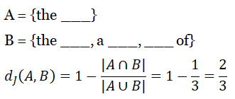
In the second example, where A has one item but B has three, the shortest possible Jaccard Distance between A and B is 2/3, a significant difference compared to the minimum distance of 0 in the first example.
The current version of the Gradient Syntactic Model will not correct for this bias. This is because, if the training corpus were large enough, the size of a word’s context set would not depend on the word’s frequency of occurrence. In an infinitely large corpus, all words, regardless of their frequencies, would occur in all the contexts allowed by the language. In that case, differences in context set size would no longer be the result of differences in word frequency, but of differences in contextual variety. This would then no longer be a bias, but a reflection of the properties of the words being compared. Although in practice all corpora are limited in size, in the end, it is still the completeness of the corpus that is the issue, and not the metric itself. Thus, the Jaccard Distance will be used without any further modifications.
⁵ ^ The Jaccard similarity coefficient

would also have served the purpose. However, distances can be mapped more easily to mathematical spaces (e.g. Euclidean space), something that may be useful in the future.
3.1.2 Evaluation
Since there are no established lexical-syntactic distances between words that can be used as a standard, the Jaccard Distance must be evaluated indirectly. One method of indirect evaluation is to use precision at k, a metric used in information theory. To measure the precision at k of the Jaccard Distances between a word (the head word) and the other words it is compared to (its neighbours), we sort the neighbours from the shortest Jaccard Distance to the farthest. Then, we compare the POS tags of the head word with the tags of each of its neighbours (a word in the Penn Treebank can have more than one tag). If a neighbour shares at least one tag with the head word, the neighbour counts as a match. Precision at k is the percentage of POS-tag matches among the k most similar neighbours. This is calculated for all values k. Ideally, all matching neighbours would be ranked at the top of the list, and precision at k would decrease monotonically.
We choose a sample of ten words from the corpus, representing ten different POS labels. These words are selected by taking the first word in the corpus that both has a context set and belongs to one of ten chosen parts of speech. The words are as follows: in (preposition), an (determiner), oct. (proper noun, specifically name of a month), 19 (numeral), review (common noun), ’s (possessive clitic), take (verb, typically transitive), steady (adjective), will (modal), and mistakenly (adverb).
The following graphs in Figure 3.1 show the precisions at k for each of the ten words:


Generally, precision peaks either at the very top of the ranking or shortly after, then drops off gradually. This is encouraging; it means that most of the neighbours that share a POS tag with the head word are near the top of the list, ranked among the head word’s most similar neighbours. Some graphs do show increases, either at the top of the ranking or near the middle. In particular, the graphs for an, steady, and mistakenly start at 0.0, then rise sharply to their peaks, before descending mostly monotonically. The graphs for 19, will, steady, and ’s show a slight increase before k=1001. 19, will, steady, and in also show a slight increase further down the ranking. This biggest anomaly is in the graph for in, which appears to consistently increase from about k=8001 until the end. However, these are minor inconsistencies; the overall trend in all the graphs is still a monotonic decrease.
Another way of assessing these rankings is to examine a small number of the neighbours with the shortest Jaccard Distances to each word. Table 3.4 show the ten nearest neighbours for each of the selected ten words. Each word is listed with all the POS tags they receive in the corpus,⁶ and each neighbour is listed with the Jaccard Distance from its head word, rounded to the nearest thousandth:
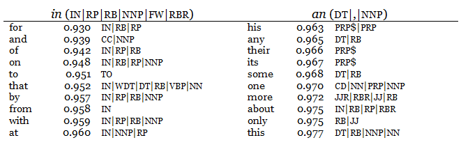


Among the lists in Table 3.4, those for oct., 19, and take contain neighbours that are especially similar. The nearest neighbours of oct. are not only proper nouns, but months of the year; the nearest neighbours of 19 are other numerals that, curiously enough, happen to be integers close to 19; and the nearest neighbours of take are verbs that are not only similarly non-third person singular present, but are also transitive. Additionally, the neighbours of take reflect the Jaccard Distance’s bias towards neighbours of similar frequency: take ranks 219th in frequency out of a total of 39,213 word types, while its nearest ten neighbours rank from 141th for make to 853th for turn.⁷ This bias is especially apparent among words in large classes like nouns and verbs, which vary greatly in frequency.
Four other lists, those for in, an, review, and will, also consist of fairly similar neighbours. The neighbours of in, like in itself, are mostly prepositions; the exceptions are and and that, which were likely judged to be similar because they are also frequently followed by nouns. The nearest neighbours of the determiner an are all words that, though not strictly determiners, function very similarly to determiners: possessors (their, its, and his), quantifiers (any, some, more, one), a preposition (about) and a predeterminer (only), and a demonstrative (this). The seven most similar neighbours of review, like review itself, are transitive verbs that can also be count nouns; the remaining three still match review by being nouns. The neighbours of review also reflect the Jaccard Distance’s frequency bias: review is ranked 1462th, while the frequency ranks of its neighbours range from 1244th for test to 3274th for consideration. Finally, among the nearest neighbours of will, nine out of ten are either modals or auxiliaries, with the sole exception of also.
Finding nearest neighbours for ’s is a more difficult task; its function as a possessive marker is already quite unique in English, let alone the combination of that function with its other duties as the contraction of is, was, and has. Three of the four nearest neighbours of ’s are the three third-person singular present verb forms, is, was, and has, which it serves as a contraction for. Five other neighbours (its, that, in, for, a) are words that, like the possessive clitic ’s, are typically followed by nouns. And and said are somewhat out of place, but they are likely present due to the fact that both, like ‘s, are also frequently found between two noun phrases.
Judging from their POS tags, the nearest neighbours of steady and mistakenly appear to be weaker matches; nevertheless, their neighbours do share some shallow similarities with their head words. The list for steady contains only three other modifiers: two adjectives (last-minute and delicate), and a participle (sagging). The rest are nouns, though second-place shot is also a verb (as the past tense and past participle of shoot). The inclusion of nouns in this list, however, is not as unreasonable as it appears: nouns and adjectives do have some contexts in common. For example, both nouns and adjectives can follow determiners (e.g. a steady stream; a conversation), although larger contexts would reveal that adjectives must eventually be followed by a noun. In fact, the only two contexts shared by the bottom eight neighbours in the list for steady are a ___ and the ___. Both nouns and adjectives can also be followed by prepositional phrases (e.g. has been steady at around 6.2%, that conversation at the residence of the U.S. ambassador). Adjectives also share contexts with past and present participles such as sagging and shot; for example, past participles can also follow the copula (e.g. was steady; was shot), while present participles can also precede nouns attributively (e.g. a steady stream; a sagging economy).
The nearest neighbours of mistakenly are worse matches than those of steady: none of them are tagged as adverbs (RB). This is partly due to the low frequency of mistakenly, which occurs only six times in the corpus (further discussion follows in the next section). Furthermore, all its contexts are derived from subsequences of a single repeated sequence, which were mistakenly shown in the quarterly earnings surprises table in. It shares only one context with each of its neighbours in the list, were ___, and this is also the only context of many of its neighbours. The relatively low similarity of the nearest neighbours of mistakenly shows that to be meaningful, lexical-syntactic similarities cannot hinge on only one context, but must be based on a large variety of contexts — the more the better.
⁶ ^ Some questionable-looking tags, such as ɴɴᴘ for and and ᴠʙ for nov., are probably due to tagging conventions in the Penn Treebank. Nevertheless, I have chosen to include them here.
⁷ ^ As previously mentioned, frequency rankings excludes all punctuation except apostrophes, $, and periods in abbreviations.
3.1.3 Discussion
The measurement of the lexical-syntactic similarity between pairs of words using the Jaccard Distance provides a viable alternative to parts of speech, with all the additional advantages of a gradient model. Precision at k results for the neighbours of a sample of ten words with diverse lexical-syntactic behaviour show that matching neighbours generally have shorter Jaccard Distances than other words. A closer examination of the lists of ten most similar neighbours for the ten words in the sample shows that Jaccard Distances has the potential to identify deep lexical-syntactic similarities.
Nevertheless, at least two of lists in Table 3.4 are somewhat weak. The number of weak matches in the top-ten neighbour lists appear to be higher for words with low frequencies. Table 3.5 shows the raw frequencies of the ten words in the evaluation sample, their frequency rankings, and the number of contexts in their context sets. The words with the most strong matches, oct. and 19, do not have the highest frequencies or the most contexts; however, those with the most weak matches, steady and mistakenly, do have the lowest frequencies and the fewest contexts. The strong matches in the lists for oct. and 19 may perhaps be due to their more restrictive contexts. In any case, the data suggests that high frequency and small context sizes, relative to the degree of contextual diversity, is a factor in the performance of the metric.

The effectiveness of the Jaccard Distance is also limited by its dependence on contexts that are both local (i.e. immediately adjacent) and purely lexical (i.e. without information about the general lexical-syntactic behaviour of the words in the contexts). While local contexts can theoretically include long-distance contextual information, longer repeated sequences are less frequent, thus making long-distance contexts more difficult to identify. A larger training corpus would boost the frequencies of all words; however, no matter how large a corpus is, Zipf’s law guarantees that it will always have a significant number of low-frequency words. A more systematic solution would be to generalize the words in a context to other similar words, so that contexts can be grouped with other similar contexts. For example, a lovely ___ and a beautiful ___ could be recognized as similar contexts, once the similarity lovely and beautiful is known to the model. This similarity, however, is the very information that the Lexical-Syntactic Similarity module is trying to gather.
One solution is to iterate the learning algorithm. By the end of one full iteration of training, the model will have acquired Jaccard Distances between all pairs of words with context sets. In a subsequent iteration, these distances could then be used to generalize each context to groups of similar contexts, thereby increasing the number of instances available to the model. This would also boost the frequency of longer contexts, thus facilitating the inference of long-distance contextual information. This in turn allows the model to update its Jaccard Distances to reflect deeper lexical-syntactic similarities. As explained in the Introduction, iterative training unfortunately lies outside the scope of the current dissertation, but will hopefully be implemented in the future.
3.2 Phrases
In its most basic sense, phrases are simply multi-word sequences that behave like a single unit. Individual words behave like a unit when they constrain each other’s behaviour. These constraints can work on different levels, phonological, morphological, syntactic, or semantic. Since the current model is a syntactic model with no access to semantics, it will regard phrases as units that impose syntactic constraints on its component words. An example of a syntactic constraint can be seen, for example, in the noun phrase these advantages. This phrase contains two constraints: the determiner these must occur before the noun advantages, and each word’s plurality must agree with the other’s.
The challenge for the model is to identify syntactic phrases without the benefit of higher-level linguistic concepts (e.g. parts of speech, plurality). In this section, we will develop a metric to measure the unit-like behaviour of phrases, using relative frequency as a starting point (Hay 2001, Bybee 2010). We will also develop two different ways of measuring degrees of similarity between phrases: by comparing their contexts (contextual similarity), and by comparing their component words (internal similarity).
3.2.1 Phrasal coherence
Phrasal coherence refers to the degree to which a phrase behaves like a unit. Since phrases can contain different numbers of constraints ― and of varying strengths ― phrasal coherence is a gradient property that should be measurable. A starting point is the idea of relative frequency, the ratio of the frequency of a morphologically-complex word to the frequency of its base (Hay 2001). In Hay (2001), high relative frequency is shown to be correlated with lower semantic transparency. Later, Bybee (2010:149) applies relative frequency to phrases, calculating the frequency of auxiliary-gerund combinations in Spanish as a percentage of either the auxiliary or the gerund.
Measuring phrasal coherence requires somewhat different information — the frequency of a phrase should be compared not to the frequency of its component words individually, but to the frequency we would expect the phrase to have if its component words occurred completely independently. This baseline frequency can be calculated by the product of the relative frequencies of its component words. The higher the observed frequency of the phrase relative to the baseline frequency, the higher its phrasal coherence.
This is somewhat similar to pointwise mutual information (PMI). In information theory, PMI is the difference in self-information between two events occurring together as a joint event, and the same two events occurring as independent events:

where x and y are two events. In a phrase, x and y would represent its component words.
Applying this formula to phrases requires two modifications. First, phrases are not just limited to two words, but can consist of any number. Second, unlike the events in PMI, words in a phrase occur consecutively, and in a specific order. This does not entail a difference in the calculation, but does nevertheless make a difference in the notation: the occurrence of the phrase in the numerator should be considered a single event, rather a joint event.
Accounting for these two considerations, the revised measure, which will be referred to as sequential pointwise mutual information (or SPMI), can be defined as
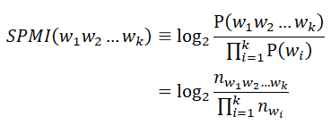
where k is the length of the phrase, wᵢ is the ith word in the phrase, and

is the frequency of the phrase in the corpus. Base-two logarithm is used, following computer science convention.
These concepts can be summed up in the following operational definition of a phrase:
Phrase —
A phrase is a sequence of more than one word, whose observed frequency in the corpus is higher than a baseline frequency where its component words all occur independently.
The degree of coherence of the phrase is measured by its sequential pointwise mutual information (SPMI), which is given by

To illustrate the kinds of phrases that have high SPMIs, Table 3.6 shows the ten phrases with the highest SPMIs of lengths two, three, and four respectively:⁸

A cursory glance reveals that almost all the phrases with the highest SPMIs, of all lengths, are proper nouns. This makes sense: many of the words that make up these sequences have very low frequencies in the corpus, which in turn leads to very low baseline frequencies for these phrases. Although the majority of the listed phrases occur only two or three times in the corpus, their low baseline probabilities result in high SPMIs.
Note that a high SPMI does not guarantee that a sequence is a complete phrase. In particular, the lists in Table 3.4 contain some phrases that are incomplete phrases, and occur only as parts of longer phrases. For example, the phrases ho chi and chi minh occur only as part of the longer phrase ho chi minh.⁹ To determine whether a phrase can occur outside of some longer phrase, we simply need to compare the frequency of the shorter phrase with that of the longer one. If the frequencies are the same, the shorter phrase can only occur as part of the longer one. For example, ho chi minh occurs twice, as does ho chi and chi minh; thus, we know that the two shorter phrases occur only as part of the longer one.
As a further illustration, we can measure the SPMIs of repeated sequences in a sentence taken from the Penn Treebank. The repeated sequences in the sentence are listed below in Table 3.7, along with their frequency counts and SPMIs. The phrases are sorted from the greatest SPMI to the least. Again, for reference, the total number of word tokens in the corpus is 933,886:

Table 3.7 shows that longer phrases tend to have higher SPMIs. This is because, as phrases grow longer, their baseline probabilities drop exponentially, since they are the product of the probabilities of all the individual words in the phrase. This bias towards longer phrases is in fact desirable: SPMIs should reflect the fact that the frequent occurrence of longer phrases is less probable, and therefore more informative, than equally frequent occurrences of shorter ones.
Unlike in conventional phrasal analyses, phrases in the Gradient Syntactic Model are not discrete units. Thus, they can partially overlap. And while some phrases are stronger than others in terms of their SPMI, they are all considered to be valid phrases, and are all part of the final analysis of the sentence.
How well do these SPMI measurements correspond to conventional expectations of which sequences should be phrases? As a comparison, the following are the phrases that would have been part of a generative phrase-structure analysis:
the luxury auto maker (NP)
luxury auto maker (N’)
auto maker (N’)
last year (AdvP)
1,214 cars (NP)
in the u.s. (PP)
the u.s. (NP)
If SPMI measures agreed with generative analyses, phrases in the generative analysis would all be at the top of the SPMI ranking, and vice versa. Two of them in fact are: the noun phrase the luxury auto maker has the highest SPMI, while the N’ that it contains, luxury auto maker, ranks second. However, there are numerous phrases for which the generative analysis and the SPMI rankings do not agree. One of these, 1,214 cars, is a phrase from the generative analysis that does not appear in the SPMI ranking. This is because it is not a repeated sequence in the corpus, most likely because of the uniqueness of the numeral 1,214. The rest of the mismatches are repeated sequences that do not appear in the generative analysis.
The main reason for the discrepancy between SPMI scores and conventional phrasal analyses is that conventional analyses are based not on the properties of particular phrases, but on the properties of types of phrases, or phrasal categories, such as noun phrases, adjective phrases, and so on. Identifying frequent phrase types yields broader syntactic patterns than identifying particular phrases. In a gradient framework, instead of using discrete phrasal categories, this can be done by identifying similar phrases, using a similarity metric akin to the lexical-syntactic similarity measure in the last section, then defining a threshold.
To this end, we must first define a measurement of phrasal similarity.
⁸ ^ All the top ten items of length 2 are tied in SPMI.
⁹ ^ Ho Chi Minh was the first president and prime minister of North Vietnam.
3.2.2 Phrasal comparison
The Lexical-Syntactic Similarity module measured the degree of similarity in lexical-syntactic behaviour between pairs of words. In the Phrases module, it is the similarity between pairs of phrases that is measured. There are two ways to compare phrases. One is contextual comparison, where the similarity between two phrases is taken to be the similarity between their context sets, as was done earlier for pairs of words. Two phrases can also be compared by internal comparison, which compares the similarity between words in the two phrase that occupy each linear position. Below, I will describe each type of comparison in more detail, as well as present their implementation and evaluation.
Contextual comparison
Contextual comparison refers to the comparison of two items by the contexts they occur in. The contextual comparison of phrases proceeds in a manner very similar to the measurement of lexical-syntactic similarity. Contexts of phrases are extracted from longer repeated sequences that contain these phrases, then blanking the phrases out. For example, to extract a context for the phrase chief executive officer from the repeated sequence president and chief executive officer, we can blank out chief executive officer in the longer sequence, to get the context president and ___. This context can then be entered into the context set of chief executive officer. Once context sets have been established for as many phrases as possible, they can be used to calculate Jaccard Distances between pairs of phrases.
To judge how well contextual comparisons of phrases align with conventional phrasal categories, we can examine the lists of most similar phrasal neighbours for a sample of five phrases, each representing one of the five main phrasal categories: noun phrase, verb phrase, adjective phrase, adverbial phrase, and prepositional phrase.
Ideally, this five-phrase sample should be chosen randomly; unfortunately, many phrases have very small context sets, which causes similarity scores to be based on very shallow similarities. As discussed previously, in a future version of the model where training consists of multiple iterations, contexts may be able to be generalized to other similar contexts using information acquired in earlier iterations. This should offset the problem of small context sets. At this stage, however, phrases with small contexts would not perform well, and would fail to accurately reflect the potential of contextual comparison.
Thus, for our evaluation, we will select phrases with adequately large contexts to represent each of the five phrasal categories: the summer (noun phrase), to find (infinitive verb phrase), more difficult (adjective phrase), very much (adverbial phrase), and in the u.s. (preposition phrase). Below are the lists of the 10 neighbours with the smallest Jaccard Distances to each of those five phrases:

Of the ten nearest neighbours of the summer, eight of them are well-formed noun phrases. Among the remaining two, 1990 because comes close to being well-formed, differing from a noun phrase only by the presence of because. Its low Jaccard Distance is most likely from sharing the context in ___ of with the head phrase, along with the two subsequence contexts in ___ and ___ of.¹⁰ The other mismatched neighbour, belgium said …, also ranks high due to the context in ___ of. Phrases such as belgium said … are problematic for contextual comparisons, because long phrases with rare structures can occasionally share an accidental context with phrases with common structures. This is similar to the problem with the measurement of lexical-syntactic similarity, which was often too heavily skewed by superficial similarities for words with low frequencies and small context sizes. Again, generalized contexts would be able to solve this problem.

The list of ten nearest neighbours of the infinitive verb phrase to find also consists mainly of phrases of the same type; all of them at least contain infinitive verb phrases. Seven are infinitive verb phrases with the exact same structure as the head phrase (to followed by a verb), while the other three contain either extra material to the right (to find a buyer for, to find offsetting cuts) or to the left (after failing to find). All three of these still contain the complete head phrase to find.

Compared to the first two lists, the list of nearest neighbours for the adjective phrase more difficult is more mixed. Of these ten neighbours, three of them (also likely, n’t able, almost certain), like the head phrase, contain an adverb followed by an adjective. Two others contain a well-matched adjective phrase, but with an extra word (more difficult to, is more difficult). Three others end with adjectives, but precede them with the copula instead of an adverb (is easy, ’s safe, is important). The remaining two consist of a verb phrase (’s trying) and a noun phrase (an embarrassment).
The greater variance in this list can be traced to at least three factors, which to some extent appear to mutually reinforce each other. First, more difficult has a small context set, with only 12 contexts (Table 3.11). Thus, many of its phrasal neighbours obtain low Jaccard Distances to it on the basis of only six widely-shared contexts that are based on only two repeated sequences: it ___ to, along with the subsequence contexts it ___ and ___ to; and is ___ to, along with is ___ and ___ to. In fact, sharing three contexts with more difficult is enough for a phrase to attain a Jaccard Distance of 0.75, which is the distance attained by the bottom eight phrases on the list.

The problem of having a small context set is exacerbated by another problem, the shared contexts themselves. The three contexts most widely-shared by the phrasal neighbours in the list, it ___ to, it ___, and ___ to, are not very selective, and can occur with a wide variety of phrases: besides adjective phrases (as in [make] it more difficult to), they can also easily accommodate verb phrases, especially those that begin with the copula (e.g. it is easy to, it is important to, it ’s safe to).
The third factor, and perhaps the more important factor in this case, is that there are few phrases with a matching POS tag sequence in the training corpus to begin with. As Table 3.11 shows, there are only 24 repeated sequences in the training corpus that share the exact POS tag sequence as more difficult, compared to 1639 for the summer and 489 for to find. With fewer matching phrases in the corpus, it becomes less likely for any one of these phrases to share many contexts with more difficult. For example, the phrase with the tag sequence ʀʙʀ ᴊᴊ that has the lowest Jaccard Distance to more difficult is the phrase less likely. Despite its similarity to the head phrase, its context set only has one context, ___ to. Although more difficult also has that context, it is a very common context, shared by many other phrases. Meanwhile, for a phrase like the summer, which has 1639 phrases with an identical tag sequence, many more of them shared enough contexts with the summer to attain the low Jaccard Distances.

The list of nearest neighbours for the adverbial (and sometimes adjective) phrase very much contain even fewer matching neighbours than more difficult. It contains just two phrases with exactly matching POS tag sequences, heavily concentrated and n’t alone. Among the rest, the closest matches are the three phrases headed by past participles: considered …, scheduled to open, and expected to begin. Since past participles often behave like adjectives, these phrases likely share contexts with the adjectival contexts of very much. The rest consist of four noun phrases, and a non-phrase that is one word off from a noun phrase (a free-lance writer based).
The reasons for the small number of matching neighbours for very much appear to be the same as those seen previously with more difficult: few matching phrases in the training corpus, small context sets, and contexts that are too common. Among phrases with context sets, only 178 match one of the two POS tag sequences of very much (63 with ʀʙ ʀʙ and 115 with ʀʙ ᴊᴊ). This is more than the 24 phrases that match more difficult, but still much fewer than the 1639 matches of the summer. As mentioned before, having a small number of matching phrases in the corpus decreases the chances that any of them will share enough contexts with the head phrase to attain a low Jaccard Distance to it. Further exacerbating the problem is the small context size of very much, which only has 7 contexts, the fewest among the five phrases being evaluated. Finally, the contexts most commonly shared by the phrasal neighbours on the list, is ___ in, together with its subsequence contexts is ___ and ___ in, can occur with phrases with a wide variety of behaviours.

The training corpus contains a number of long repeated sequences, and the subsequences that they contain also become repeated sequences. Here, a number of them have risen to the top of the list as the closest neighbours of in the u.s. Of the ten phrases listed, the top eight phrases (nine including the u.s.) are merely subsequences of just two long repeated sequences: in the u.s. using the same questionnaire, and in the u.s. and non-u.s. capital markets. These phrases attain low Jaccard Distances because they all share the same, and often very specific, left contexts (e.g. survey every household ___) as the head phrase. Similarly, the phrase the u.s. appears in the list mostly because it shares many specific right contexts with the head phrase.
We can try to remedy this by pruning subsequence contexts. The resulting list of nearest neighbours would then look like this:

The list is now free of those redundant subsequences of long repeated sequences containing the head phrase. There are now four unique prepositional phrases in the list, all of which are at the very top. The fifth-ranked phrase, last month, is a time adverbial, which behaves much like prepositional phrases. The bottom half of the list, however, is somewhat disappointing: apart from one noun phrase (the issue), the rest are all non-phrases.
With in the u.s., the presence of rather poor matches in the bottom half of the list cannot be traced to a small context set; its context set contains 249 contexts, by far the most among the five phrases evaluated here. Nor is the number of similar phrases in the training corpus particularly small. The difficulty seems to lie elsewhere.
Three related factors appear to contribute to the difficulty of making contextual comparisons with prepositional phrases like in the u.s. First, prepositional phrases can occur in a wide range of contexts. This makes it less likely that any two prepositional phrases will share the same context. Since adverbs and adverbial phrases also occur in a wide range of contexts, this factor is also likely behind the relatively poor matches among the closest neighbours of the phrases more difficult and very much. Second, when a prepositional phrase does share a context with another phrase, the context is often too common, admitting too many different kinds of phrases. Among the contexts shared by in the u.s. and its neighbours, many are purely right contexts consisting of prepositions, the conjunction and, and forms of the verbs have and be. Such contexts can fit almost any phrase. Finally, many of the contexts of in the u.s. that its closest neighbours in Table 3.14 do not share are too specific. The words adjacent to the head phrase in these contexts are too low in frequency to be applicable to very many other phrases; examples include slowdown ___ economy and an unexpectedly sharp widening ___ trade gap. If the model could generalize these contexts to other syntactically-similar contexts, the closest neighbours of in the u.s. might consist of more prepositional phrases, or at least phrases with more deeply similar behaviour.
The solutions to all these problems are the same as those proposed for poor matches in lexical-syntactic similarity. A larger corpus would likely lead to some improvement. However, it is likely more effective to iterate the training process, so that similar contexts can be identified and used together, their applicability can be broaden, and longer contexts can be identified.
Internal comparison
In addition to comparison by context, phrases can also be compared by their internal structures. For example, phrases consisting of a determiner followed by a noun (e.g. the company, a book, this place) share a similar internal structure; at each word position, they are made up of words with similar lexical-syntactic behaviour. Although internal comparison does not compare the contexts of phrases, phrases with similar internal structure nevertheless have a strong tendency to occur in similar contexts. Phrases consisting of a determiner and a noun, such as those just listed, almost always occur in contexts typical of nouns.
One way to compare two phrases internally, if they each contain the same number of words, is to calculate the Jaccard Distance between the words in each linear position, position-by-position, then adding the resulting similarities into a single similarity measurement. This measurement can be referred to as sequential distance.
In practice, there is a problem with calculating the sequential distance by simply adding these raw Jaccard Distances: the differences between large and small Jaccard Distances are often too small to significantly affect the final sum. For example, in the evaluation of the Jaccard Distance in the first module, the most similar neighbour of in was for, with a Jaccard Distance of 0.930. This leaves only a difference of 0.07 between the most similar neighbour and the most dissimilar word possible, which would have a Jaccard Distance of 1.0. It is a difference that can be easily drowned out by noise elsewhere in the phrase. Additionally, the neighbours of different words have different ranges of Jaccard Distances. While the closest neighbour of in has a Jaccard Distance of 0.930 with it, the transitive verbs replace and affect (Table 3.3) have a Jaccard Distance of 0.741. This disparity can make comparisons very unpredictable.
Therefore, in order to have an informative sequential distance, we need to exaggerate the difference between the Jaccard Distances of similar and dissimilar neighbours. One way to do this is to transform Jaccard Distances by taking the difference between 1 and the Jaccard Distance, then taking the reciprocal of that distance, or

The lowest value of this transformed Jaccard Distance would be 1, when xᵢ and yᵢ are identical, while the highest score would be unlimited, when xᵢ and yᵢ share no contexts. This means that some phrases can have infinite sequential distances; however, this is not a problem, since the model is concerned with identifying the most similar phrases, not the most dissimilar ones.¹¹
Thus, we arrive at the following definition of sequential distance:
Sequential distance –
The sequential distance between two sequence of words, x and y, each of which contains the same number of words, is the sum of the reciprocal of the Jaccard similarity (one minus the Jaccard Distance) between the word from x and the word from y at each word position. That is,

where xᵢ and yᵢ are the words at position i in the phrases x and y respectively, and dᴊ(xᵢ,yᵢ) is the Jaccard Distance between them. A low seqdist value indicates that a pair of phrases are sequentially similar.
To illustrate with an example, consider the phrases in the u.s. and on a computer. To measure the sequential distance between them, the words in each phrase are compared position-by-position, so that in is compared with on, the is compared to a, and u.s. is compared to computer. Applying the formula above to the two phrases, we get the following:

Thus, the sequential distance between in the u.s. and on the computer is 66.673.¹² To provide a reference point for this raw sequentially distance, if the phrase on the computer were actually in the corpus, it would have the 690th lowest sequential distance to the phrase in the u.s., out of 54,241 three-word phrases in the corpus (in other words, within the top second percentile).
The fact that on the computer is not a phrase in the training corpus illustrates how sequential distances can be calculated between two phrases that do not appear in the corpus. As long as every word in both phrases have context sets, the Jaccard Distances between words in each word position can be calculated, and from there the sequential distance of the phrases can also be calculated.
Since the sequential distance is not normalized for phrase length, it tends to assign shorter sequential distances to shorter phrases. Since sequential distances are only calculated between phrases of identical lengths, this length bias is not an issue when differentiating between neighbours of the same phrase. However, when comparing the closeness of the neighbours of different phrases, sequential distances should be normalized for length.
To judge how well sequential distances align with conventional linguistic analysis, we can repeat the methodology from the contextual comparison section, and examine the most similar phrasal neighbours of a selection of five phrases, one from each of five phrase types: the role (noun phrase), has n’t been set (verb phrase), partly responsible (adjective phrase), more closely (adverbial phrase), and in the u.s. (prepositional phrase). These five phrases are the first instance of each phrase type in the corpus that contains only words with context sets. Listed below are the ten most similar phrasal neighbours for each of the phrases, with their sequential distances (rounded to the nearest thousandth), their normalized sequential distances, and their POS tags:

The top ten matches for the noun phrase the role are all noun phrases with very similar phrase structures. All consist of a determiner followed by a noun; nine of these nouns are even singular. All of these phrasal neighbours, like the head phrase, also begin with the same determiner the, thereby keeping down the sequential distance considerably. Additionally, with a large number of nouns in the corpus, there is also a correspondingly large number of nouns that occur in many of the same contexts as role. This is in positive contrast to the problematic situation seen earlier with more difficult and very much.

Overall, the ten closest neighbours of the verb phrase has n’t been set are also quite similar to their head phrase, even if they are not as similar as the closest neighbours of the role. The second token in all neighbours is the contraction n’t. Among the top five phrases, the third words are also identical to the third word in the head phrase, while the first words are either identical or an inflectional variant (have). Only the fourth words shows more variety, with two being past participles like in the head phrase, one present participle, and two occurrences of the adjective able. Among the bottom five phrases in the list, three still begin with has or have, but two are the modals could and would; these modals are functionally similar to has. The third words in the sixth and seventh phrases are still past participles, but become the infinitive be in the eighth and ninth phrases, and an adverb in the last. The raw sequential distances of these phrasal neighbours are significantly higher than those of the role, but are more similar after being normalized for length.

At a glance, the closest neighbours of partly responsible appear comparable in quality to those of has n’t been set. The sequential distances reflect this: after being normalized for length, they are comparable to those of the phrases in the middle range of the list for has n’t been set.
A large majority of the phrases in Table 3.17 consist of an adverb followed by either an adjective or a verbal participle, past or present. The sole exception is remains responsible, which begins with a verb instead of an adverb; it was likely judged to be similar because it shares the second word responsible with the head phrase, and because remains, like many adverbs, often occurs in front adjectives.

By sequential distance, the closest neighbours of the adverbial phrase more closely (Table 3.18) are even more similar to the head phrase more closely than the neighbours of the role are to their head phrase. However, qualitatively, they appear less similar. The sequential distances of all ten phrases are kept low by sharing the first word more. The second words, however, are either adjectives or nouns; none are adverbs like closely.
Examining the profiles of closely and those of the second words of the phrasal neighbours in the list, we see that many of the contexts they share can accommodate adverbs, adjectives, and nouns alike; examples include a ___, the ___, of ___, is ___, and more ___ to. Since all three parts of speech can occur at the beginning of noun phrases, they can also all follow determiners, prepositions such as of, and the copula. The context more ___ to can also take words from all three categories. In short, the sequential distances attained by the neighbours of more closely are low primarily because their second words share exceedingly common contexts with the word closely.

With few exceptions, most of the nearest neighbours of in the u.s. are similarly made up of a preposition, the determiner the, and a noun, in that order. The exceptions for the first word are and and that; previously in the Lexical-Syntactic Similarity module, we have seen that and and that are sometimes judged to be similar to prepositions because they are both often followed by nouns. The second words of the phrasal neighbours are all identical to the second word of the head phrase, the. The third word is a noun in eight of the phrases in the list, six of which have the identical word as the head phrase, u.s. The two non-nouns are the adjectives japanese and federal; the similarity between adjectives and nouns has also been observed before in the previous module, since both nouns and adjectives follow determiners as well copulas.
Despite the presence of a few questionable matches, the normalized sequential distances of the phrases in this list are comparable to the lists for the role and more closely. Like the neighbours of more closely, those of in the u.s. still register low sequential distances because they share identical words with their head phrase. Because each word position is treated independently in the calculation of sequential distance, this gives leeway for other words in the phrase to differ more, while still keeping the sequential distance low. This issue may become less pronounced when the training process becomes iterative, and when Jaccard Distances between words can more accurately reflect deeper lexical-syntactic similarities. However, it is also possible that this may be an inherent shortcoming in the way sequential distance is currently calculated. This issue merits further investigation.
¹⁰ ^ Subsequence contexts refer to contexts created from subsequences of a longer repeated sequence. In this case, in the summer is a subsequence of the repeated sequence in the summer of, making in ___ a subsequence context of in ___ of. Subsequence contexts count the same as other contexts in the calculation of Jaccard Distances.
¹¹ ^ There is also the possibility that two very similar phrases can have an infinite sequential distance because one of the phrases has a word that shares no contexts with the corresponding word in the other phrase, something that can easily happen. This goes back to the problem of inadequate contexts, which is addressed elsewhere in this chapter.
¹² ^ Though the Jaccard Distances shown in the formula have been rounded, the resulting sequential distance of 66.673 has been calculated with unrounded values.
3.3 Conditional probabilities
The third and final module of the Gradient Syntactic Model, Conditional Probabilities, identifies predictive relationships between pairs of elements. The training algorithm estimates the probability of occurrence of each element (which, again, is either a word or phrase) found in the training corpus, given the occurrence of a second element occurring in the same sentence, in a specific position relative to the first. We will call the first element the predicted element, and the second one the given element. Either element can also alternatively be replaced in the conditional event by its neighbourhood, a group consisting of the elements most similar to it.
These conditional probabilities indicate how strong syntactic patterns are. Taken together, the conditional probabilities in a sentence can be used to calculate the predictability of the entire sentence. This leads to the idea of calculating a grammaticality score based on the sum of all the conditional probabilities between all pairs of elements. A sentence’s grammaticality score thus becomes a measure of the fit between the sentence and the syntactic model learned from training. A sentence with a high grammatical score is one that contains the most and strongest syntactic patterns known to the model. Conversely, the best-fitting syntactic model for a set of grammatical sentences is the one that assigns them the highest grammatical scores.
In this section, we will first develop a precise definition of the conditional events whose probabilities are estimated in this module. Then, we will a develop a grammaticality score and describe how it is calculated. Finally, to illustrate the application of these concepts, we will calculate the conditional probabilities and the grammaticality score of a selection of sentences not in the training corpus. We will observe how well grammaticality scores can differentiate between grammatical and ungrammatical sentences, and also compare conditional probabilities with conventional discrete syntactic analyses.
3.3.1 Conditional probabilities
Predictability is central to the notion of grammaticality. While language contains much that is unpredictable — indeed it is in its unpredictability that new information can be expressed — it also contains many patterns that are predictable. The predictable allows listeners to decode the unpredictable, and to understand the new information it carries.
Each syntactic pattern can be modeled as a conditional event, where the occurrence of one element, the predicted element, is predicted by the occurrence of another element in the same sentence, the given element. The probability predicted element is also affected by its linear position relative to the given one. This information can be captured by two variables: direction, the direction of the predicted element relative to the given element, with left and right as the possible values; and distance, the absolute difference between the word positions of predicted element and the given element (e.g. adjacent elements are separated by a distance of 1). When at least one of the two elements is a phrase, the word in each element closest to the other element is used; for example, two adjacent phrases are separated by a distance of 1.
Thus, each of these conditional probabilities takes the form
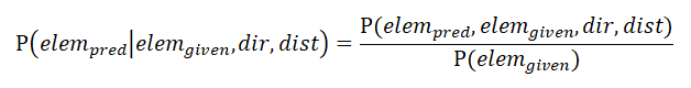
where elemₚᵣₑ is the predicted element, elemᵢᵥₑₙ is the given element, dir is the direction of elemₚᵣₑ relative to elemᵢᵥₑₙ, and dist is the distance between them, (given by the absolute difference between the linear positions of the closest words they contain). For example, from the noun phrase the sun, we can formulate the conditional probability P(“sun”|“the”,right,1); this is the probability of sun, given the occurrence of the to the immediate right of the. An example of a conditional probability involving phrases can be illustrated by the sentence the president arrived in the afternoon. We can be formulate a conditional probability between the phrases the president and in the afternoon: if the president is the predicted element, the conditional probability would be P(“the president”|“in the afternoon”,left,2). Note that although in this conditional probability these two phrases appear to be discrete entities, they still exhibit gradient variation in their phrasal coherence, as measured by SPMI.
In addition to estimating conditional probabilities between individual words or phrases, we can also estimate conditional probabilities between their neighbourhoods, or sets consisting of an element plus some of its nearest neighbours. Conditional probabilities involving these neighbourhoods can be written as

where neigh(x) represents all the elements in the neighbourhood of element x, , including x itself. For example, from the noun phrase the sun, we can formulate the conditional probability P(neigh(“sun”)|neigh(“the”),right,1). This is the probability of occurrence of the any word in the neighbourhood of sun, given that it occurs immediately to the right of any word in the neighbourhood of the.
Neighbourhoods can be defined in at least three ways: 1) by imposing a hard threshold; 2) by assigning different weights to different neighbours, according to their distances from the head element; or 3) both. Theoretically, assigning weights to neighbours is the more principled method; it requires no arbitrary cut-off point, it does not create a binary division between neighbours and non-neighbours, and it recognizes the different degrees of similarity among the neighbours. However, the assignment of weights requires more computation, and some experimentation to find an appropriate weighting scheme. Since the development of the Gradient Syntactic Model is still in its early stages, we will first resort to the simpler strategy of setting a hard threshold: neighbourhoods of words will consist of words with a Jaccard Distance of 0.95 or lower, and neighbourhoods of phrases will consist of words with a sequential distance of 30.0 or lower. The use of weights can be explored in the future.
3.3.2 Grammaticality
In a natural linguistic community, grammaticality refers to the degree to which an utterance conforms to the community’s norms of language usage. Their expectations are formed over their lifetimes, from exposure to the language around them. In the Gradient Syntactic Model, the norms of language usage are inferred from a training corpus, by measuring properties associated with the behaviours of the language’s words and phrases: lexical-syntactic similarity between words and phrases, phrasal coherence, and the conditional probabilities between words and phrases. Thus, the grammaticality of a sentence (or any word sequence) becomes a measurement of how well it conforms to the model’s expectations.
This leads to the idea of measuring the grammaticality of a sentence using a grammaticality score that measures the total strength of the syntactic patterns in the sentence. The more syntactic patterns the model recognizes, and the higher these probabilities are, the more closely the word sequence can be said to conform to the model. We can then calculate the grammaticality score of a sentence by summing up all significant conditional probabilities in the word sequence. This grammaticality score is analogous to the use of Gross Domestic Product (GDP) to measure the strength of a country’s economy: each conditional probability between two elements in a word sequence corresponds to the purchase of a good or service produced within a country. Additionally, since longer word sequences contain more recognizable patterns than shorter ones, grammaticality scores should be normalized by the length of the word sequence, just as GDP per capita is the GDP normalized by a country’s population. A formula for such a grammaticality score would thus look like this:

where x and y are either elements or neighbourhoods of elements occuring in the same sentence, and length(W) is the number of words in W.
Before this formula is ready for use, it requires three adjustments. First, the significance of a high conditional probability depends on how frequent the predicted element is by itself. Thus, the conditional probabilities of x in the summation should be normalized by x’s a priori probability, P(x).¹³ The resulting ratio, P(x|y,…)/P(x), can be referred to as the conditional probability ratio. Note that this ratio is the same when the predicted element and the given element are switched:

Second, only conditional probability ratios that indicate a significant predictive relationship between two elements should be included in the calculation of the grammaticality score. Among pairs of adjacent elements, only those that occur in the same sentence more often than random will be included; that is, their conditional probability ratios must be greater than one. Among pairs of non-adjacent elements, the constraint must be stricter; without constraints on their linear positions, pairs of elements may appear frequently in the same sentence because of semantic reasons rather than syntactic ones. Thus, the grammaticality score will only include pairs of non-adjacent elements that occur in the same sentence more frequently than random, at every distance shorter than their distance in the current sentence. For example, if a pair of elements have a conditional probability ratio greater than one when separated by a distance of three, their ratios must also be greater than one when they are separated by a distance of two, and also when they are adjacent to each other.
Finally, the grammaticality score should use the logarithms of conditional probability ratios. This is because the ratios can in practice vary over many orders of magnitude; for example, the greatest ratio between a pair of words is 2¹⁸·⁸³³, while the smallest value is 2⁻⁸·⁷¹¹. Only by taking the logarithm of the ratio can we prevent pairs of elements with very strong values from overwhelming the contribution of other pairs of elements in the sentence. Following the precedent we set with the definition of SPMI, we will use a base-two logarithm.
We are now ready to define the grammaticality score:
Grammaticality score –
The grammaticality score of a word sequence W with respect to a grammatical model M, or G(W|M), is given by

where x and y are non-overlapping elements (or the neighbourhoods of these elements) in W, dir(x,y,W) is the direction of x’s position relative to y in W, dist(x,y,W) is the absolute difference in word position between x and y in W, length(W) is the number of words in W, and S is the set containing all pairs (x,y) such that
- each pair is only counted once in S,
i.e. if (x,y) ∈ S then (y,x) ∉ S; - conditional probability ratios of adjacent elements must exceed one,
i.e. P(x|y,dir(x,y,W),dist(x,y,W))/P(x) > 1, if dist(x,y,W) = 1; - conditional probability ratios of non-adjacent elements must exceed one for all distances less than and including dist(x,y,W),
i.e. P(x|y,dir(x,y,W),dist(x,y,W))/P(x) > 1,
∀ dist(x,y,w) s.t. dist(x,y,w) ≤ dist(x,y,W), if dist(x,y,W) = 1
To illustrate the calculation of the conditional probability ratio, P(x|y,dir(x,y,W),dist(x,y,W))/P(x), consider a pair of words taken from one of the sentences in the training corpus: those and who, in the sentence not all those who wrote oppose the changes. To calculate P(“those”|“who”,left,1)/P(“those”), we need four numbers: the raw frequency of those in the corpus, n(“those”), which is 567; the frequency of who (1580), the frequency of the bigram those who (61), and the total number of words in the corpus (933,886). From this, we can calculate the ratio:

Thus, those occurs immediately in front of who 63.589 times more often than it does in general. The base-two logarithm of the ratio is 5.991.
The calculation of grammaticality scores makes use of much (though not all) of the information in the Gradient Syntactic Model: lexical-syntactic similarities between pairs of elements are captured by the inclusion of neighbourhoods; phrases are identified by matching them to repeated sequences in the training corpus; and of course, conditional probabilities. Thus, to an extent, the grammaticality score can be considered the assessment of a sentence by the Gradient Syntactic Model as a whole.
One of the few pieces of information from the model not directly used in the calculation of the score is SPMI, the measurement of phrasal coherence. However, we can show that the information expressed by SPMIs is actually indirectly conveyed by the conditional probabilities, at least for phrases of length two. To do this, we compare the formula for the conditional probability ratio between two adjacent elements to the formula for SPMI for phrases of length two.
Since

given a two-word phrase w₁w₂, we have:

This shows that the SPMI for phrases consisting of two words is actually equal to the conditional probability ratio between these two words.
In the next section, we will evaluate how well grammaticality scores align with the grammaticality of language in common use.
¹³ ^ The a priori probability of x is x’s probability before knowing any other information about it.
3.3.3 Evaluation
To see how well grammaticality scores correspond to the grammaticality of commonly-used language, we will calculate the grammaticality scores of a number of grammatical sentences, and contrast them with the grammaticality scores of the same sentences after their words have been randomly rearranged. If grammaticality scores reflect the expectations of English speakers, they should be markedly different in the grammatical sentences compared to the ungrammatical ones.
The test sentences are taken from the New York Times. The sentences are chosen to be fairly short, being no more than 11 words long. This is both to ensure the results are not too complicated to interpret, and to minimize the processing time needed to produce them. For similar reasons, the number of test sentences will be kept at 20 (10 grammatical and 10 ungrammatical). Additionally, because the Gradient Syntactic Model cannot infer information about out-of-vocabulary items, all the words in the test sentences must not only appear in the training corpus, but must also already have context sets.
The 20 test sentences (minus punctuation) are

Producing a grammaticality score for a sentence consists of 1) identifying the phrases in the sentence; 2) finding the neighbourhoods of all its words and phrases; and 3) calculating the conditional probability ratios between all pairings of words, phrases, neighbourhoods of words, and neighbourhoods of phrases in the sentence, a total of ten types of pairings. We can illustrate this entire process with the first test sentence, Sentence 1 (they thought it would never happen). The phrases are simply the repeated sequences in the sentence. Table 3.21 is a list of the phrases in Sentence 1, along with word-position indices, their frequencies in the training corpus, and their SPMIs:

The following tables give the logged conditional probability ratios between the pairs of elements or neighbourhoods of elements in Sentence 1, rounded to the nearest thousandth. Only ratios that meet the conditions for inclusion in the calculation of the grammaticality score are shown. Dashed lines ( — ) indicate overlapping or identical elements. Thresholds for neighbourhoods are a maximum Jaccard Distance of 0.95 for words, and a maximum sequential distance of 30.0 for phrases.


Summing up all the logged conditional probability ratios and dividing the sum by the number of words in the sentence (6), we obtain a grammaticality score of 32.147.
Applying the same analysis to all ten sentence pairs yields the following grammaticality scores for all 20 test sentences:


As Table 3.23 and Figure 3.3 show, for all ten pairs of test sentences, the grammaticality scores of the grammatical sentences are significantly greater than that of their corresponding ungrammatical sentences, ranging from 2.05 times greater in Pair 7 (Sentences 13 and 14) to 8.48 times greater in Pair 8 (Sentences 15 and 16). The lowest grammaticality score among grammatical sentences is still higher than the highest grammaticality score among ungrammatical sentences.
Despite the length-normalization already included in the calculation of the grammaticality score, there is still a noticeable effect of length on grammaticality scores, especially for grammatical sentences. Ideally, if length were to have no effect whatsoever, the correlation should be zero. Here, the correlation is 0.375 for all sentences, 0.290 for the grammatical sentences, and 0.099 for the ungrammatical sentences. If grammaticality scores are to be comparable across sentences of various lengths, an adjustment may be necessary in their formula. This should be investigated more thoroughly in the future.
While grammaticality scores provide a succinct assessment of the a sentence’s grammaticality, it is also useful to have an overall view of its grammatical patterns. This can be provided by a visual representation of grammatical patterns that is in some ways comparable to the visual representations of phrase-structure and dependency analyses.
For easier comparison with discrete analyses, gradient analyses need to represent only ratios between pairs of neighbourhoods. This is because typically, discrete syntactic analyses treat lexical items only as representatives of their categories, rather than as individual items. A noun phrase such as the tree would be labeled as an NP in a phrase-structure tree, and the noun tree would be labeled the head of the, without any consideration to any idiosyncrasies this particular phrase might have. Such an approach focuses on the most general –and for descriptive linguistics, the most important — syntactic patterns in a language. It is important to keep in mind, however, that even though the gradient visual representation only displays some of the conditional probability ratios, those not shown are nevertheless still important parts of a complete syntactic analysis in the Gradient Syntactic Model.
The visual representation for the analysis of Sentence 1 looks like this:

Rectangular boxes are drawn around all phrases. Lines are used to represent all conditional probability ratios between pairs of neighbourhoods (i.e. two neighbourhoods of words, two neighbourhoods of phrases, or the neighbourhood of a word with the neighbourhood of a phrase) that are included in the calculation of the grammaticality score. Lines above the sentence represent ratios between neighbourhoods of words, while lines below the sentence represent ratios involving neighbourhoods of phrases. The darkness of the line is proportional to the base-two log of the ratio, up to a maximum of 5.0. Since conditional probability ratios are the same even if the predicted element and the given element are switched, the lines representing these ratios are non-directed.
It should be expected that the gradient analyses of the evaluated sentences will be quite different from their discrete analyses, for several reasons. First, the phrases and conditional probabilities in the gradient analyses differ from phrase structures and dependency relations in important ways. Whereas phrases in conventional phrase structures are phrasal categories, phrases in the current gradient model are repeated sequences. And whereas dependency relations in conventional dependency graphs use head words to represent larger phrases, the gradient analysis allow phrases to simply represent themselves. Second, as discussed before, the current implementation is limited both by a relatively small training corpus and by the execution of only one training iteration. A more fully-developed version of the model may be able to assess the strengths of syntactic patterns more accurately, producing gradient analyses that align more closely with conventional expectations. Finally, while discrete analyses tend to represent only the strongest relationships, gradient analyses include all conditional probability ratios greater than 1 (or greater than 0 when logged). This often results in visual representations that seem overwhelmingly complex. However, it must be remembered that the Gradient Syntactic Model is designed not for humans, but for machines, and not for simplicity, but for detail and precision. Rather than striving for neatness, the strategy of the Gradient Syntactic Model is to include both strong and weak syntactic patterns, and to let the stronger ones emerge naturally.
Despite these significant divergences, it is instructive to compare the gradient analyses of the ten grammatical sentences in this evaluation with their corresponding discrete analyses. These discrete analyses will consist of both phrase structures and dependency relations that, for ease of comparison, will be combined into a single visual representation. Phrases are not labeled with phrasal categories, and dependency relations are not marked for direction, since phrases in gradient analyses have no labels either, and lines representing conditional probability ratios are non-directed. Otherwise, they represent the same information as phrase-structure trees and dependency graphs. For example, the following is the discrete analysis of Sentence 1:

Phrases are marked in rectangular boxes. Because the dependencies are between pairs of words, they are marked above the sentence, with non-directed lines.
We can now examine the visual representations of the analyses of the 20 chosen sentences (with discussion to follow):
Pair 1
Sentence 1
Gradient analysis

Discrete analysis
Sentence 2
Gradient analysis

Pair 2
Sentence 3
Gradient analysis

Discrete analysis
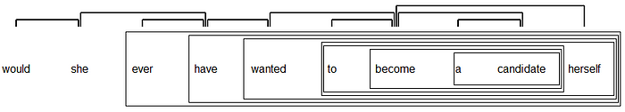
Sentence 4
Gradient analysis

Pair 3
Sentence 5
Gradient analysis

Discrete analysis

Sentence 6
Gradient analysis

Pair 4
Sentence 7
Gradient analysis

Discrete analysis

Sentence 8
Gradient analysis

Pair 5
Sentence 9
Gradient analysis

Discrete analysis

Sentence 10
Gradient analysis

Pair 6
Sentence 11
Gradient analysis

Discrete analysis

Sentence 12
Gradient analysis

Pair 7
Sentence 13
Gradient analysis

Discrete analysis

Sentence 14
Gradient analysis
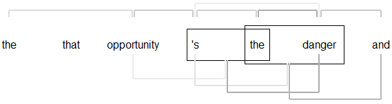
Pair 8
Sentence 15
Gradient analysis

Discrete analysis

Sentence 16
Gradient analysis

Pair 9
Sentence 17
Gradient analysis
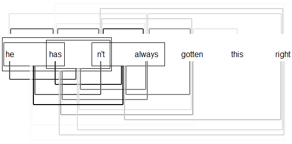
Discrete analysis

Sentence 18
Gradient analysis

Pair 10
Sentence 19
Gradient analysis

Discrete analysis

Sentence 20
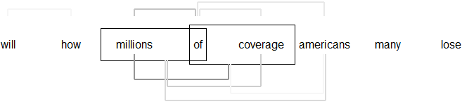
As expected, the gradient analyses of the grammatical sentences differ greatly from their discrete counterparts. Nevertheless, we can still make a number of high-level qualitative observations. One immediate observation is the noticeably greater density of the lines and boxes in the grammatical sentences, compared to the ungrammatical ones. These visual representations are thus able to show the contrast between the density of syntactic patterns in different parts of a sentence. For example, although it is an ungrammatical sentence, Sentence 8 does contain a grammatical sequence in its latter half, but the shift in that is clear. The model identifies significantly more patterns in this grammatical portion of the sentence than in the previous part, offing seems it a, which is more clearly ungrammatical.
A second observation is that most of the ratios in the gradient analyses are between adjacent elements, whether they be adjacent words, words adjacent to phrases, or adjacent phrases. Ratios between elements with distances of two or greater tend to be lower (represented by fainter lines) compared to those between adjacent elements. This predominance of local patterns emerges naturally, despite the fact that conditional probability ratios were calculated between all pairs of elements in the sentence.
These analyses also reveal flaws in the current version of the model. For example, several grammatical sequences should contain more recognized patterns than they currently do. For example, in Sentence 9, this nightmare is completely bare; it is not marked as a phrase, nor are there any conditional probabilities involving the neighbourhoods of its component words. It is perhaps somewhat expected that it would not marked as a phrase, since many phrases are not frequent, and therefore would not be a repeated sequence in the training corpus. However, it is more surprising that the neighbourhood of neither word is included in any conditional probabilities. The main reason for this is that this only has one neighbour (last) with which it has a Jaccard Distance less than or equal to the threshold of 0.95, leaving it with only one word in its neighbourhood. This confirms our earlier suspicions that using such hard thresholds is a crude method of defining neighbourhoods.
Another area for improvement in the gradient analyses that has been made obvious by this comparison with discrete analyses is in the identification of phrases. Currently, the phrases in the gradient analyses are merely repeated sequences from the training corpus; the model has not used similarity measurements between words or phrases to identify frequent phrasal neighbourhoods. It is these frequent phrasal neighbourhoods that would be the gradient equivalents of phrasal categories (e.g. noun phrases, verb phrases, adjective phrases), which — casting their drawbacks as categories aside for the moment — do reveal deep syntactic patterns that repeated sequences simply cannot.
Despite their complexity, visual representations of gradient analyses provide a quick way for humans to identify syntactic patterns in sentences. Additionally, compared to the simpler visual representations of discrete analyses, they have the advantage of showing precisely-defined patterns. Finally, it should be remembered that the Gradient Syntactic Model is not primarily designed for human consumption. The complexity of the model’s analysis should pose no problems for the computer applications that it is ultimately meant for.
4 Conclusions
The Gradient Syntactic Model provides an alternative to the discrete syntactic models still commonly used in unsupervised parsing algorithms. This dissertation lays down the theoretical foundation for the model, remaking the high-level discrete concepts of parts of speech, phrases, dependencies, and grammaticality into precisely-defined gradient concepts. It also implements this model computationally, trains it on a text corpus, presents results, and evaluates them both qualitatively and quantitatively.
In this final chapter, I will first summarize the major innovations of the model, then discuss possible directions for its development in the future.
4.1 Contributions
The Gradient Syntactic Model is a promising yet concrete alternative to the conventional discrete syntactic models still prevalent in unsupervised parsing and in linguistics. To unsupervised parsing, the model offers rich quantitative data that describes syntactic patterns in all their gradient complexity, using precise definitions. To linguistics, the model provides a rigorous theoretical framework that enables quantitative observations about syntax beyond frequency counts, where claims about syntactic phenomena can be tested.
The model has three major general advantages over discrete models. First, it is able to capture variations that discrete models fail to capture: differences in degree of lexical-syntactic similarity between words within the same part of speech, and similarities between words in different parts of speech; differences in coherence among phrases; and differences in prediction strength between pairs of elements in a sentence. Second, the concepts used in the Gradient Syntactic Model are simpler and more precisely-defined than those of discrete models. This is possible precisely because of the gradience allowed by the model. Third, whereas parts of speech, constituencies, and dependencies are typically learned separately, the Gradient Syntactic Model learns them together, recognizing how closely intertwined they are with each other. Measurements of lexical-syntactic similarity are used to compare phrases, while similarity scores both between words and between phrases are used to form neighbourhoods, which are then included in conditional probabilities.
Each module in the model remakes a different concept in discrete syntactic models. The Lexical-Syntactic Similarity module replaces parts of speech with a single metric that measures the degree of lexical-syntactic similarity between pairs of words, providing a more complex view of lexical-syntactic behaviour. The method of extracting contexts from repeated sequences is another innovation, deviating from past POS-induction algorithms where contexts come from a fixed number of adjacent words on either side of a target word. The results here are encouraging: many of the nearest neighbours of evaluated words are similar in lexical-syntactic behaviour, often with matching POS tags. Precision at k shows that most of the neighbours with matching POS tags are ranked among the most similar.
The Phrases module replaces constituents and diagnostic tests for constituency with phrases that, at least at this stage, are simply repeated sequences in the training corpus; phrases that capture the same general syntactic patterns that constituents do will be discussed as part of future work in the next section. Meanwhile, repeated sequences still form an important part of the whole syntactic picture. The model differentiates these repeated sequences by their degrees of phrasal coherence, as measured by a new metric, Sequential Pointwise Mutual Information (SPMI). SPMI calculates how many times more frequent a phrase occurs compared to the frequency it would have if all its component words occurred independently. In addition, the module describes two methods of phrasal comparison, contextual comparison and internal comparison. In contextual comparison, the context sets of two phrases are compared in the same way that pairs of words are compared in the Lexical-Syntactic Similarity module. In internal comparison, a sequential distance is calculated between two phrases from the Jaccard Distances between their component words in each linear position. Though only evaluated on a small scale, both methods show encouraging results, with internal comparisons performing better overall. A major impediment appears to be data sparsity; strategies for alleviating this problem will be discussed in the next section.
Finally, the last module remakes dependency relations into conditional probabilities between pairs of elements, or their neighbourhoods, that occur in the same sentence. These probabilities are conditioned not only on the occurrence of a given element or its neighbourhood, but are also conditioned on the position of the predicted element relative to it. These probabilities are then used to calculate grammaticality scores for sentences. These grammaticality score are able to clearly distinguish between grammatical and ungrammatical sentences: the scores of ten chosen grammatical sentences are between two to more than eight times higher than the scores of the ungrammatical scrambled versions of these sentences. In addition, conditional probabilities can also be used to construct a visual representation of grammatical patterns within a sentence, thereby revealing which parts of the sentence contain a greater density of grammatical patterns than others. Thus, conditional probabilities allow the expression of a clearer and more complex notion of grammaticality than has been possible before.
The Gradient Syntactic Model offers a promising starting point for a new type of syntactic model, and a new approach to the problem of unsupervised parsing. Now that a basic framework of the model has been established, it can be extended towards greater functionality.
4.2 The road ahead
The current version of the Gradient Syntactic Model qualifies as a basic foundation, but is by no means complete. There are numerous possible extensions that can improve it substantially, some of which take little effort relative to their potential payoff. The most important improvements are 1) eliminating hard thresholds in the definition of neighbourhoods; 2) phrases that capture general syntactic patterns; 3) using a larger corpus; 4) iterating the training process; 5) inferring the behaviours of new elements; and 6) extending analysis to morphological and phonological patterns.
The first three of these improvement pertains to specific parts of the model. One of these is the use of hard thresholds to define neighbourhoods for words and phrases in the Conditional Probabilities module. The threshold of 0.95 for Jaccard Distances between words and the threshold of 30.0 for sequential distances between phrases have been carefully chosen after an examination of the data, but are nevertheless arbitrary and not theoretically well-motivated. Consequently, some neighbourhoods may be too large, or more problematically, too small (as seen in Sentence 9 in Figure 3.6). The most thorough solution is perhaps to eliminate the thresholds, and instead to indicate the membership of each neighbour in a neighbourhood using numerical weights. These weights would take into account both the raw distance between the neighbour and the head word or phrase, and the neighbour’s ranking among all the neighbours. As discussed before, this method is more computationally-expensive, but it may well be worth it.
Another specific area of improvement is the identification of frequent phrasal neighbourhoods in the Phrases module. While repeated sequences should be kept in the model, there is also a need to identify the most frequent phrasal structures in the language. The model can already identify phrasal neighbourhoods for specific phrases; it now needs only to do so for all phrases, then determine which phrasal neighbourhoods are the most prevalent in the training corpus. However, the task is complicated by the goal of defining neighbourhoods using weights instead of hard thresholds. Finding a correct way of identifying the most prevalent phrasal neighbourhoods will require some thought, and some experimentation.
A more general improvement, and perhaps the simplest improvement with the largest potential performance gain, will likely come with training the model using a significantly larger corpus. During the prototyping of the model, a smaller corpus was more convenient, hence the choice of the relatively small Penn Treebank, with just under 1 million words; in contrast, the English Gigaword Fifth Edition contains over 4 billion words. Now that the skeleton of the model has been established, we can better assess the full potential of the model by training it with larger corpora. The training process does make substantial demands on both processing and memory; however, with the cost of both being currently very low, and with some further optimization of the training process, this should not be a difficult problem.
A more substantial extension is the iteration of the training process. So far, only one iteration of training has been implemented. In the beginning of this first iteration, no information is available other than the unannotated training corpus. In the second iteration, however, the model can make use of the patterns learned from the first one: phrases, lexical-syntactic similarities between words and phrases, word and phrasal neighbourhoods, and conditional probabilities. This information can, for example, allow the model to generalize over similar contexts, thereby making them more effective in identifying similar words and phrases.
Another extension to the model with a potentially large payoff is the ability to infer the behaviours of words or phrases for which the model has no information. This functionality is crucial to the model’s handling of novel test sentences, as well as of the low-frequency elements in the corpus. This inference is only possible after the first iteration of training, after context sets have been constructed for the words and phrases that occur in repeated sequences. In subsequent iterations, the contexts of unseen elements can be matched either to a context identified in the first iteration, or to a generalized context inferred early on in a subsequent iteration.
Finally, the last major extension is the construction of a morphological and phonetic/phonological model. Thus far, the Gradient Syntactic Model only captures patterns among words. While this may be adequate for more analytic languages, it is most likely inadequate for morphologically-richer languages. Because words can have many morphological forms in such languages, the average frequency of a word form will be rather low. The ability to infer morphological relationships thus appears necessary. Additionally, with the inclusion of morphology, the need for the modeling of phonological patterns follows close behind, since many morphological patterns trigger phonological variation. Given this, there may be a possible benefit in representing input text as phonological transcriptions, rather than in the language’s traditional orthography. The possibility of inferring morphological relationships in the model also raises the possibility of eliminating word boundaries. Ultimately, natural language has no word boundaries, and thus a model that does not rely on them would be more free from arbitrary analytical decisions.
The increasing prevalence of computational analysis in linguistics has brought linguistics to the cusp of a paradigm shift. At the end of this shift, the complexities of natural language — not only its syntax, but also its morphology and phonology — will no longer be simplified to discrete concepts in order to suit our limited human comprehension, but will be given the respect it demands, through the use of precise quantitative models. Unsupervised parsers, which have thus far borrowed discrete syntactic models from linguistics, now provide the impetus to help linguists transcend them. It is my fervent hope that the work described in this dissertation can facilitate this progress.
References
Beck, D. (2002). The typology of parts of speech systems: The markedness of adjectives. New York: Routledge.
Berg-Kirkpatrick, T., Bouchard-Côté, A., DeNero, J., & Klein, D. (2010). Painless Unsupervised Learning with Features. Proceedings of NAACL 2010, (pp. 582–590). Los Angeles.
Biemann, C. (2006). Unsupervised Part-of-Speech Tagging Employing Efficient Graph Clustering. Proceedings of COLING ACL 2006 (pp. 7–12). Morristown, NJ: Association for Computational Linguistics.
Blunsom, P. (2004, August 19). Hidden Markov Models. Retrieved from http://digital.cs.usu.edu/~cyan/CS7960/hmm-tutorial.pdf
Bod, R. (2009). From Exemplar to Grammar: A Probabilistic Analogy-Based Model of Language Learning. Cognitive Science, 752–793.
Brown, P. F., Della Pietra, V. J., deSouza, P. V., Lai, J. C., & Mercer, R. L. (1990). Class-based n-gram models of natural language. Proceedings of the IBM Natural Language ITL, (pp. 283–298). Paris.
Bybee, J. (2010). Language, Usage and Cognition. Cambridge: Cambridge University Press.
Christodoulopoulos, C., Goldwater, S., & Steedman, M. (2010). Two Decades of Unsupervised POS induction: How far have we come? Proceedings of EMNLP 2010 (pp. 575–584). Association for Computational Linguistics.
Clark, A. (2000). Inducing syntactic categories by context distribution clustering. Proceedings of CoNLL-LLL, (pp. 91–94).
Deerwester, S., Dumais, S. T., Furnas, G. W., Landauer, T. K., & Harshman, R. (1990). Indexing By Latent Semantic Analysis. Journal of the American Society For Information , 391–407.
Do, C. B., & Batzoglou, S. (2008, August). What is the expectation maximization algorithm? Nature Biotechnology, 26(8), 897–899.
Finch, S., & Chater, N. (1992). Bootstrapping syntactic categories using statistical methods. In W. Daelemans, & D. Powers, Background and Experiments in Machine Learning of Natural Language (pp. 229–236). Tilburg: ITK.
Goldwater, S., & Griffiths, T. (2007). A fully Bayesian approach to unsupervised part-of-speech tagging. Proceedings of ACL 2007, (pp. 744–751). Prague, Czech Republic.
Graca, J., Ganchev, K., Taskar, B., & Pereira, F. (2009). Posterior vs parameter sparsity in latent variable models. In Y. Bengio, D. Schuurmans, J. D. Lafferty, C. K. Williams, & A. Culotta (Ed.), Proceedings of Advances in Neural Information Processing Systems 22 (NIPS 2009), (pp. 664–672).
Haghighi, A., & Klein, D. (2006). Prototype-driven learning for sequence models. Proceedings of NAACL 2006, (pp. 320–327). Morristown, NJ.
Hay, J. (2001). Lexical frequency in morphology: is everything relative? Linguistics, 39, 1041–70.
Johnson, M. (2007). Why doesn’t EM find good HMM POS-taggers? Proceedings of EMNLP-CoNLL 2007, (pp. 296–305).
Klein, D., & Manning, C. D. (2004). Corpus-Based Induction of Syntactic Structure: Models of Dependency and Constituency. Proceedings of ACL 2004.
Klein, D., & Manning, C. D. (2005). Natural language grammar induction with a generative constituent-context model. Pattern Recognition, 38(9), 1407–1419.
Klein, Dan; Manning, Christopher D. (2002). A Generative Constituent-Context Model for Improved Grammar Induction. Proceedings of ACL 2002, (pp. 128–135). Philadelphia.
Matilal, B. K. (1990). The word and the world: India’s contribution to the study of language. Oxford University Press.
Mel’cuk, I. A. (1988). Dependency Syntax: Theory and Practice. Albany, NY: State University of New York Press.
Merialdo, B. (1994, June). Tagging English Text with a Probabilistic. Computational Linguistics, 20(2), 155–171.
Radford, A. (1988). Transformational Grammar: A First Course. Cambridge: Cambridge University Press.
Redington, M., Chater, N., & F. S. (1998). Distributional Information: A Powerful Cue for Acquiring Syntactic Categories. Cognitive Science, 22(4), 425–469.
Rosenberg, A., & Hirschberg, J. (2007). V-measure: A conditional entropy-based external cluster evaluation measure. Proceedings of EMNLP-CoNLL 2007, (pp. 410–420).
Schütze, H. (1995). Distributional part-of-speech tagging. Proceedings of EACL 1995 (pp. 141–148). Morgan Kaufmann Publishers Inc.
Schütze, H., & Walsh, M. (2008). A graph-theoretic model of lexical syntactic acquisition. Proceedings of EMNLP 2008 , (pp. 917–926). Honolulu.
Seppänen, A., Rhonwen, B., & Trotta, J. (1994). On the so-called complex prepositions. Studia Anglia Posnaniensia, 29, 3–29.
Spitkovsky, V. I., Alshawi, H., & Jurafsky, D. (2010). From Baby Steps to Leapfrog: How “Less is More” in Unsupervised Dependency Parsing. Proceedings of NAACL 2010, (pp. 751–759).
Spitkovsky, V. I., Alshawi, H., & Jurafsky, D. (2011). Punctuation: Making a Point in Unsupervised Dependency Parsing. Proceedings of CoNLL, (pp. 19–28).
Spitkovsky, V. I., Alshawi, H., & Jurafsky, D. (2012). Bootstrapping Dependency Grammar Inducers from Incomplete Sentence Fragments via Austere Models. Proceedings of ICGI 2012.
Spitkovsky, V. I., Alshawi, H., & Jurafsky, D. (2013). Breaking Out of Local Optima with Count Transforms and Model Recombination: A Study in Grammar Induction. Proceedings of EMNLP 2013, (pp. 1983–1995).
Spitkovsky, V. I., Alshawi, H., Chang, A. X., & Jurafsky, D. (2011). Unsupervised Dependency Parsing without Gold Part-of-Speech Tags. Proceedings of EMNLP 2011, (pp. 1281–1290).
Wittgenstein, L. (1953). Philosophical Investigations. New York: Macmillan.
